Image segmentation
Where do we need segmentation?
- Medical imaging
- Autonomous driving
- Agriculture/Phenotyping
- Robotics
- Video analysis
- Content editing
- …
Types of segmentation
Semantic segmentation: Label each pixel with a class (no instance separation).
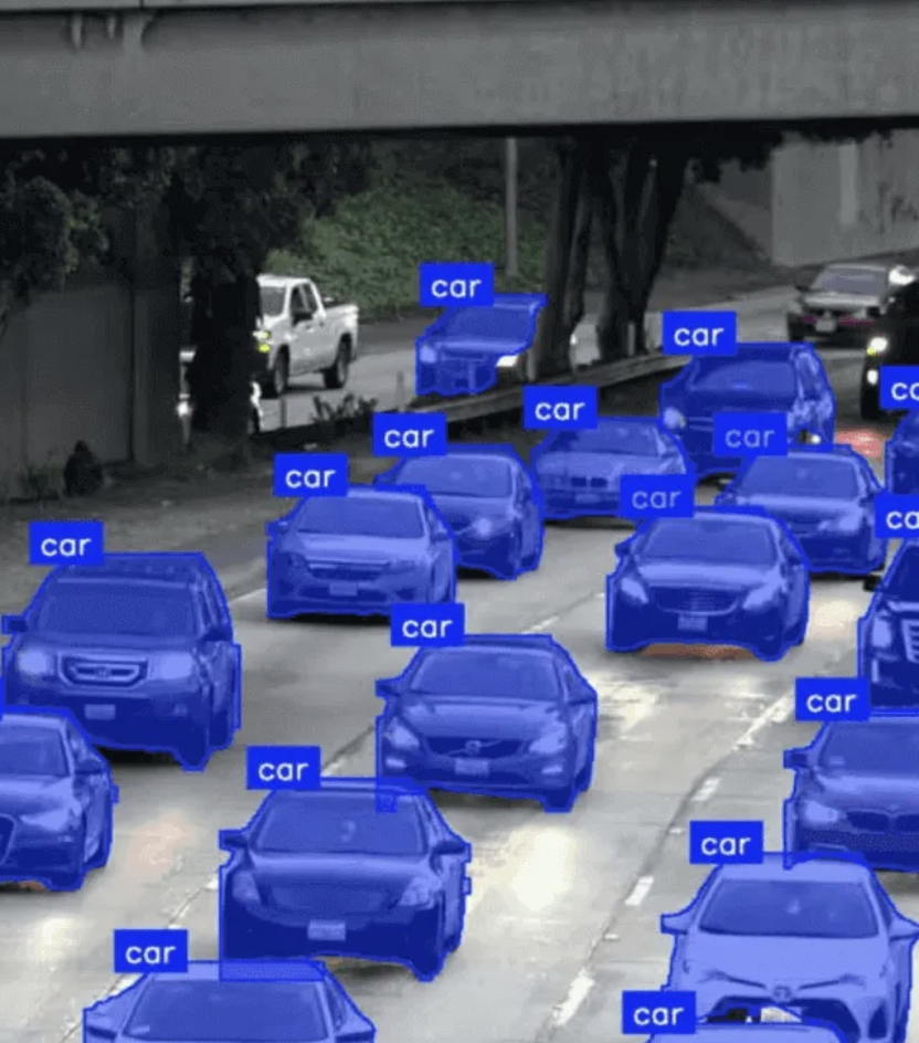
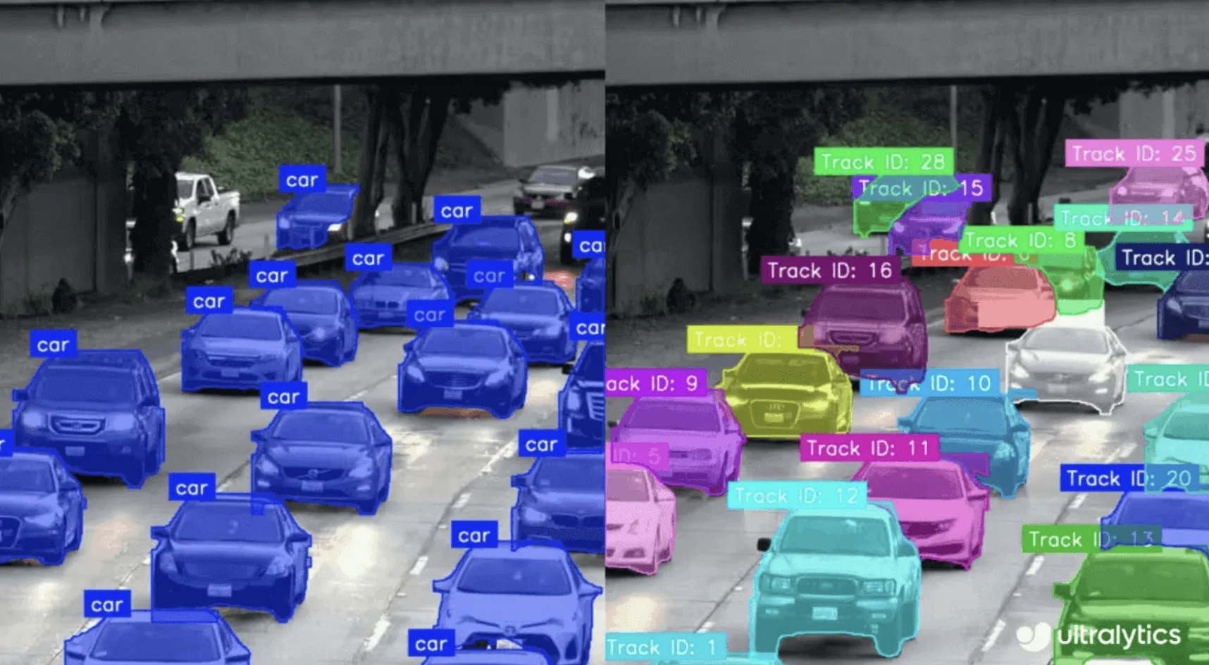
Instance segmentation: Distinguish individual objects of the same class.
Panoptic segmentation: Combines semantic + instance into one unified output.
Annotation tools

LabelMe: Web-based tool for creating polygonal and freehand annotations. Supports exporting to multiple formats like JSON for machine learning pipelines.
CVAT (Computer Vision Annotation Tool): Powerful open-source platform for image and video annotation. Supports polygons, masks, and tracking for object detection and segmentation.
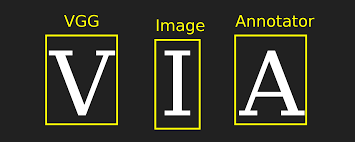
VIA (VGG Image Annotator): Lightweight, browser-based tool. Ideal for quick annotations with minimal setup. Exports annotations in JSON or CSV.
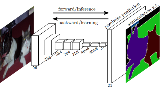
Fully convolutional networks (2015)
FCNs are a great starting point: understanding how they transform and upsample feature maps to make dense predictions provides insight into the mechanisms used in many modern image generation models.
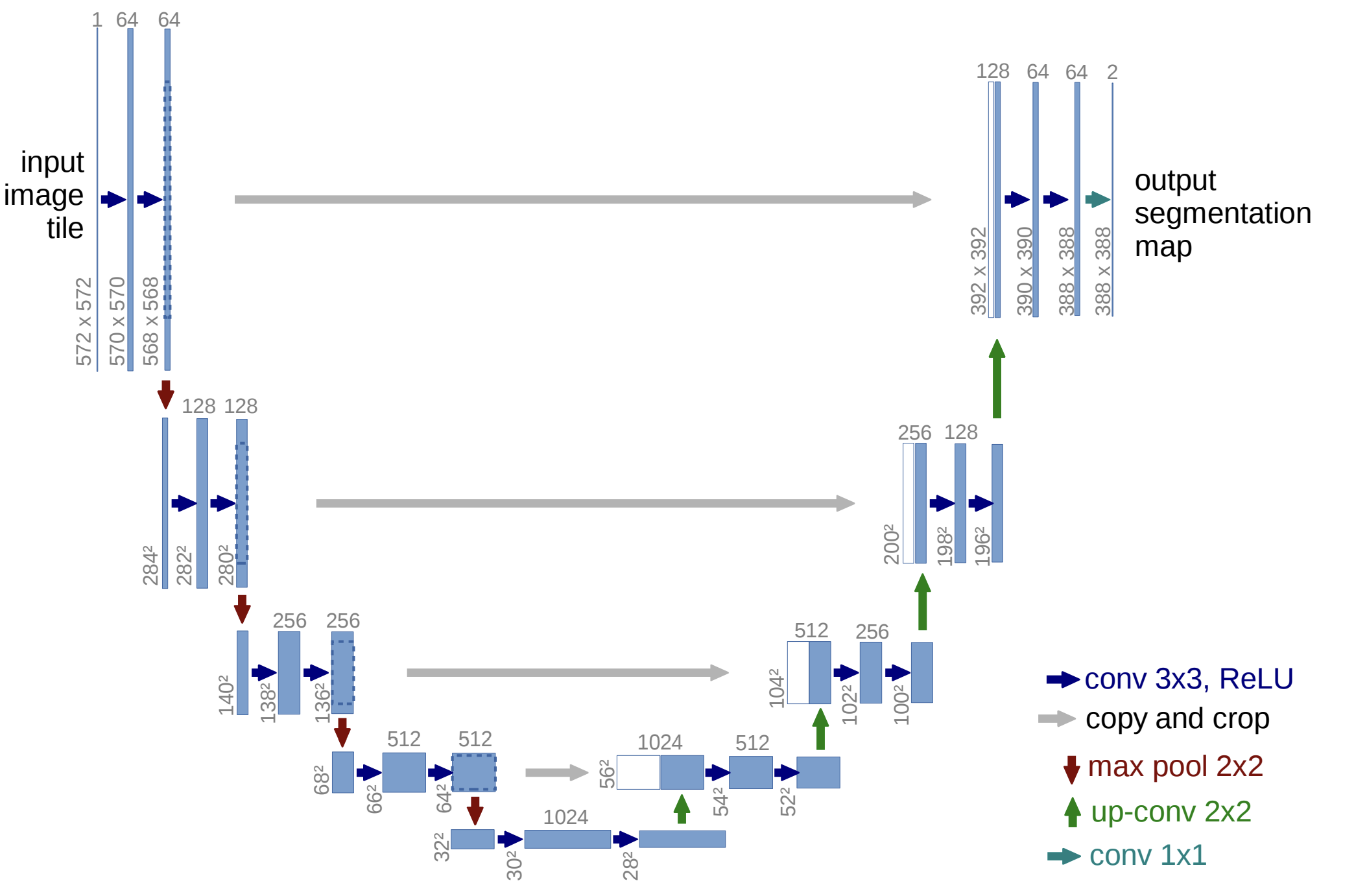
U-Net family (2015 - present)
YOLOv8 segmentation
YOLO <- ultralytics$YOLO
model <- YOLO("yolov8n-seg.pt")
result <- model$predict("slide_figures/original.png")
image 1/1 /Users/patrickli/Desktop/rproj/ibsar-cv-workshop/instructor/slides/slide_figures/original.png: 640x448 1 cat, 45.2ms
Speed: 1.5ms preprocess, 45.2ms inference, 1.1ms postprocess per image at shape (1, 3, 640, 448)'slide_figures/cat_segmentation.png'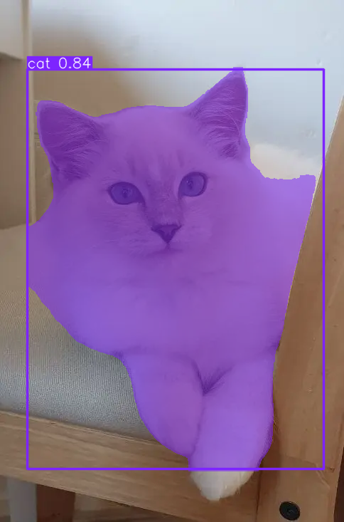
Thanks!