Deep Learning and Computer Vision in R: A Practical Introduction (4)
BIBC2025 workshop - Object Detection
Patrick Li
RSFAS, ANU
Content summary
- Overview of computer vision (CV)
reticulatebasics- Image classification
- Hyperparameter tuning
- CV model interpretation
- > Object detection
- Image segmentation
Object detection
Object detection
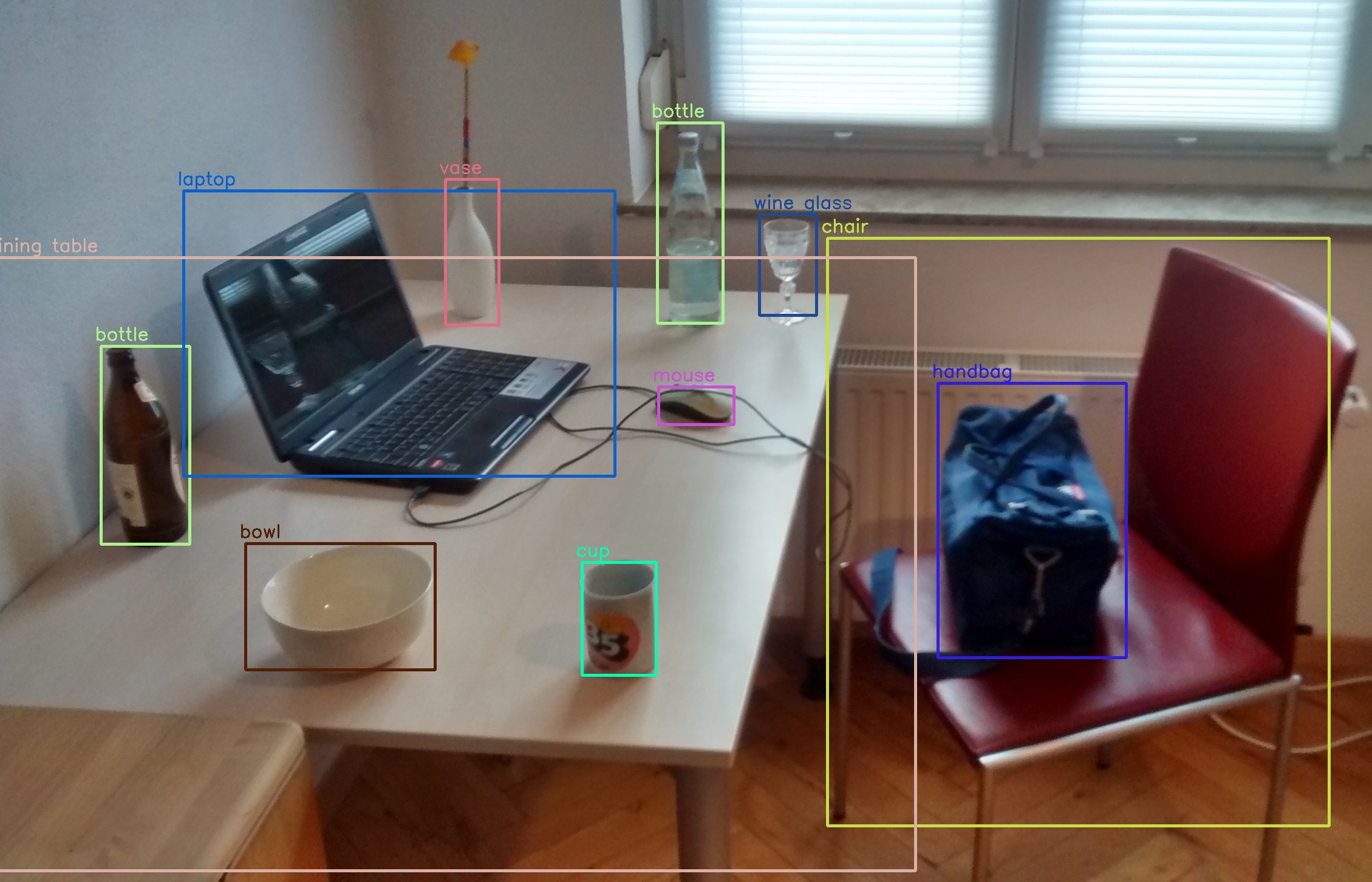
Object detection is the task of identifying and locating multiple objects within an image.
It builds on classification and localization.
- Classification: assign one label to entire image.
- Localization: predicting a single bounding box for a specific class within the entire image.
Outputs: bounding boxes + class labels + confidence scores
Why classification comes first
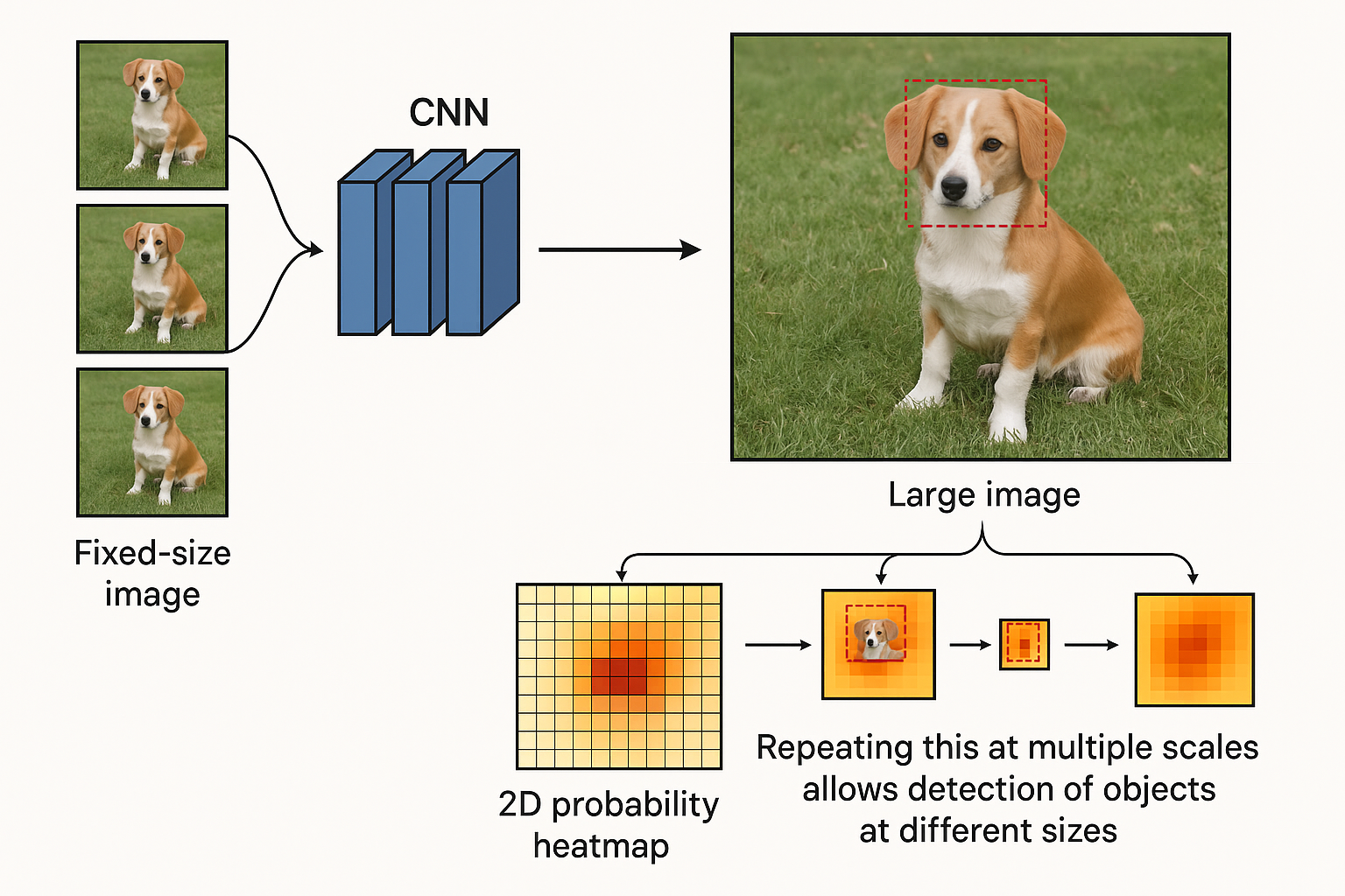
Early detection models relied on sliding-window classification, while some modern object detectors build upon pre-trained classification models.
Understanding object class features is the foundation for detection.
Challenges in object detection
Scale variation: Objects may appear very small or very large, making it hard to capture all necessary details.
Occlusion and crowding: Objects can be partially blocked or tightly packed, creating ambiguous visual cues.
Background clutter: Busy or noisy backgrounds can mislead the detector and cause false positives.
Domain shift (lighting, camera, viewpoint, scene): Models trained in one setting may not generalize well to different environments.

Data formats
There are many formats for object detection datasets, with the most common being YOLO and COCO.
For training, we need the following:
Image path (input)
One or more bounding boxes, each containing:
(x, y, w, h),(x, y)can represent either the center or the top-left corner- Class label
YOLO format
COCO format
In the COCO format, all annotations are provided in a single JSON file.
images: containsid,file_name,width,heightannotations:bbox = [x_min, y_min, width, height]category_id
categories: list of object categories
Convert COCO to YOLO format
YOLO format is simpler to use when focusing on object detection, and the ultralytics library provides a convenient way to convert COCO annotations to YOLO format.
Evaluation metrics
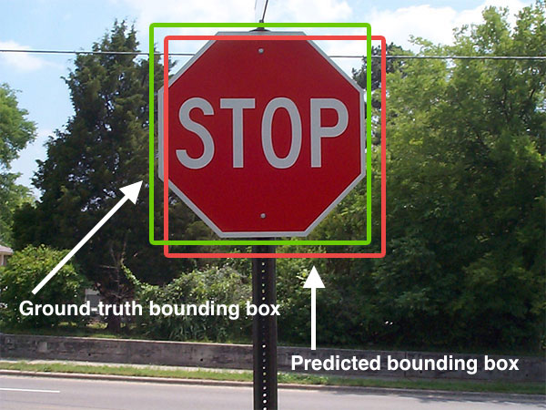
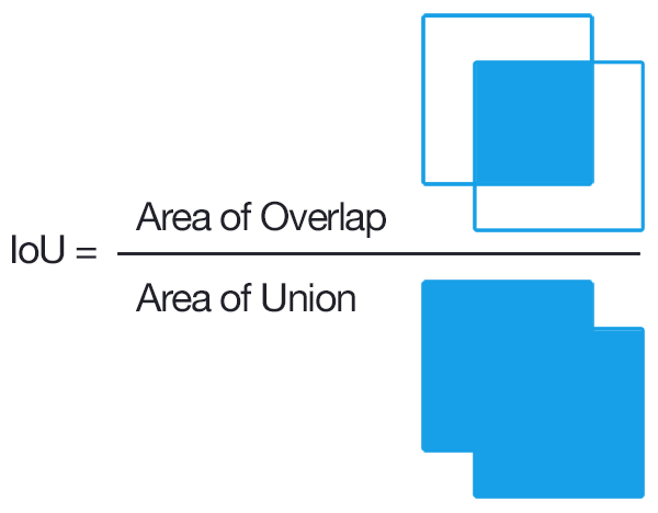
Since we are now dealing with multiple class labels and need to assess how closely a bounding box matches the ground truth, the evaluation metrics become slightly more complex.
Intersection over Union (IoU) measures how well a predicted bounding box overlaps with the ground truth.
True positive and false positive
A true positive is a predicted bounding box that satisfies all of the following:
- predicted class = ground truth class.
- IoU \geq threshold (e.g., 0.5).
- Each ground truth bounding box can be matched with at most one true positive prediction.
A false positive is a predicted bounding box that satisfies one of the following:
- Predicted class \neq any ground truth class.
- IoU < threshold for all ground truth boxes of that class.
- The ground truth box has already been matched to another true positive prediction with higher confidence score.
True negative and false negative
In object detection, true negatives are usually not counted in standard metrics, because the background (areas with no object) is vast and not explicitly evaluated.
If a ground truth bounding box does not match any predicted bounding box, it is counted as a false negative.
Precision and recall
- Precision: fraction of predicted boxes that are correct
\text{Precision} = \frac{TP}{TP + FP}
- Recall: fraction of ground truth boxes that are detected
\text{Recall} = \frac{TP}{TP + FN}
Average precision
Average precision (AP) is the area under the precision-recall (PR) curve for a single class. The PR curve is obtained by plotting the model’s precision and recall values as a function of the model’s confidence score threshold.
Mean average precision (mAP) is the average of AP over all classes:
\text{mAP} = \frac{1}{K}\sum_{k=1}^{K}AP_k
It captures overall performance across all classes.
R-CNN family
The R-CNN family, including R-CNN, Fast R-CNN, and Faster R-CNN, represents a class of two-stage detectors, where the model first generates region proposals and then classifies and refines them.
- R-CNN (2014):
- Ross Girshick (UC Berkeley), Jeff Donahue, Trevor Darrell, Jitendra Malik
- Fast R-CNN (2015)
- Ross Girshick (Microsoft Research)
- Faster R-CNN (2015)
- Shaoqing Ren, Kaiming He, Ross Girshick (Microsoft Research), Jian Sun
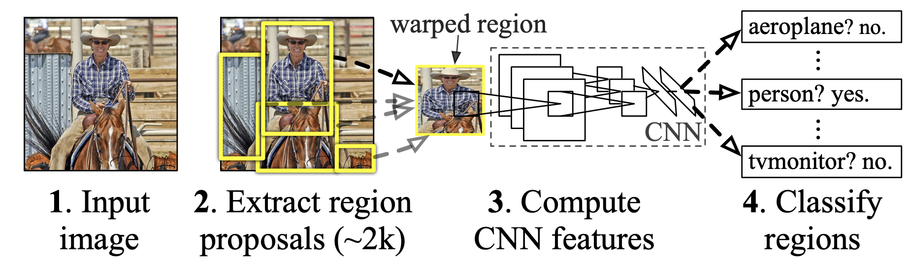
R-CNN (2014): region proposals
R-CNN generates region proposals and classifies each one using a separate CNN forward pass, achieving high accuracy but at very high computational cost.
Around 2000 region proposals are generated using Selective Search:
- Over-segment the image into many small regions (superpixels).
- Extract features for each region, including color, texture, size, and shape.
- Hierarchical grouping: recursively merge similar regions based on feature similarity.
- Select proposals: choose ~2000 regions and create bounding boxes that fully enclose the merged regions.
R-CNN (2014): detection head
For each region proposal, a pretrained CNN is applied to extract convolutional features (without using the classifier). These features are then used to train an SVM for each class. Additionally, bounding-box regression is performed using the same convolutional features to refine the predicted locations.
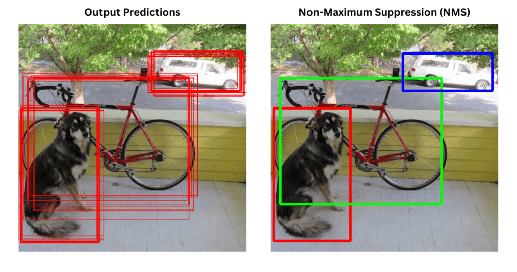
R-CNN (2014): NMS
Since region proposals can overlap, multiple predictions may correspond to the same object. To resolve this, Non-Maximum Suppression (NMS) is applied.
For each class, overlapping boxes (IoU \geq threshold) with lower confidence scores are suppressed, leaving a single, most confident bounding box per object. This reduces redundancy and improves detection precision.
Fast R-CNN (2015)
Fast R-CNN processes the entire image through a CNN to generate shared feature maps, then uses RoI pooling to classify and refine each region proposal in a single, end-to-end trainable stage.
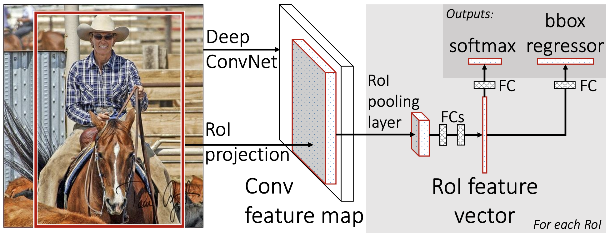
Fast R-CNN (2015): RoI pooling
Step 1: Obtain region proposals (same as R-CNN).
Region of interest (RoI) Pooling:
- Project proposal coordinates onto the CNN feature map.
- Divide each region into a fixed 7 × 7 grid.
- Apply max pooling within each grid cell.
Outcome: Fixed-size feature representation for each region, regardless of its original size.
Final Stage:
- Compute class confidence scores.
- Perform bounding-box regression for location refinement.
Faster R-CNN (2015)
Faster R-CNN introduces a Region Proposal Network (RPN) to generate region proposals directly from feature maps, eliminating the need for external methods like selective search.
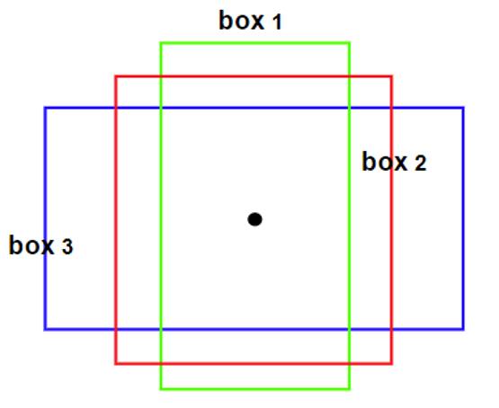
Faster R-CNN (2015): anchor box
Anchor boxes are predefined bounding boxes of various scales and aspect ratios placed at a certain position.
They are used as reference templates for the region proposal network (RPN) to predict object presence and refine box coordinates, allowing the model to handle objects of various sizes and shapes efficiently.
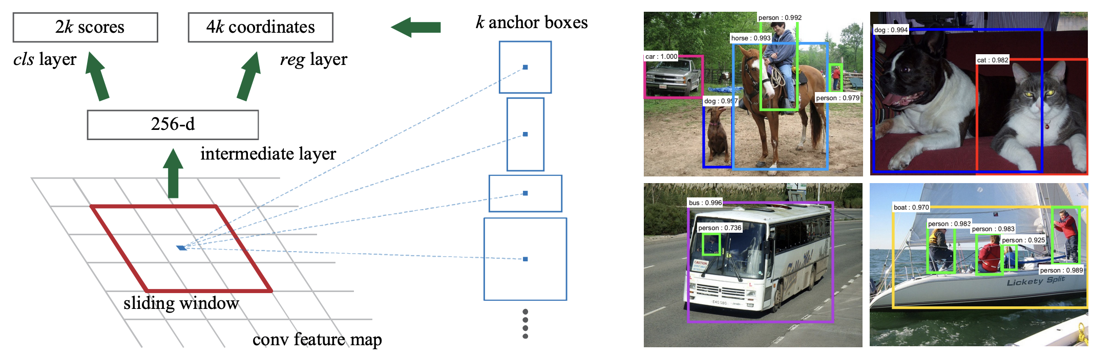
Faster R-CNN (2015): RPN
The Region Proposal Network (RPN) operates on convolutional feature maps.
At each feature map location:
- Predicts 2k objectness scores indicating whether each of k anchor boxes contains an object.
- Predicts 4k values for anchor box offsets and scales.
Anchor boxes are centered at every feature map position.
Allows efficient, end-to-end region proposal generation.
The rest of the pipeline is largely the same as Fast R-CNN.
YOLO family
YOLO (“You Only Look Once”) is a well-known family of single-stage detectors, meaning they predict bounding boxes and classes in one pass without a separate region proposal step.
| Version | Year | Authors |
|---|---|---|
| YOLOv1 | 2016 | Joseph Redmon, Santosh Divvala, Ross Girshick, Ali Farhadi |
| YOLOv2 | 2017 | Joseph Redmon, Ali Farhadi |
| YOLOv3 | 2018 | Joseph Redmon, Ali Farhadi |
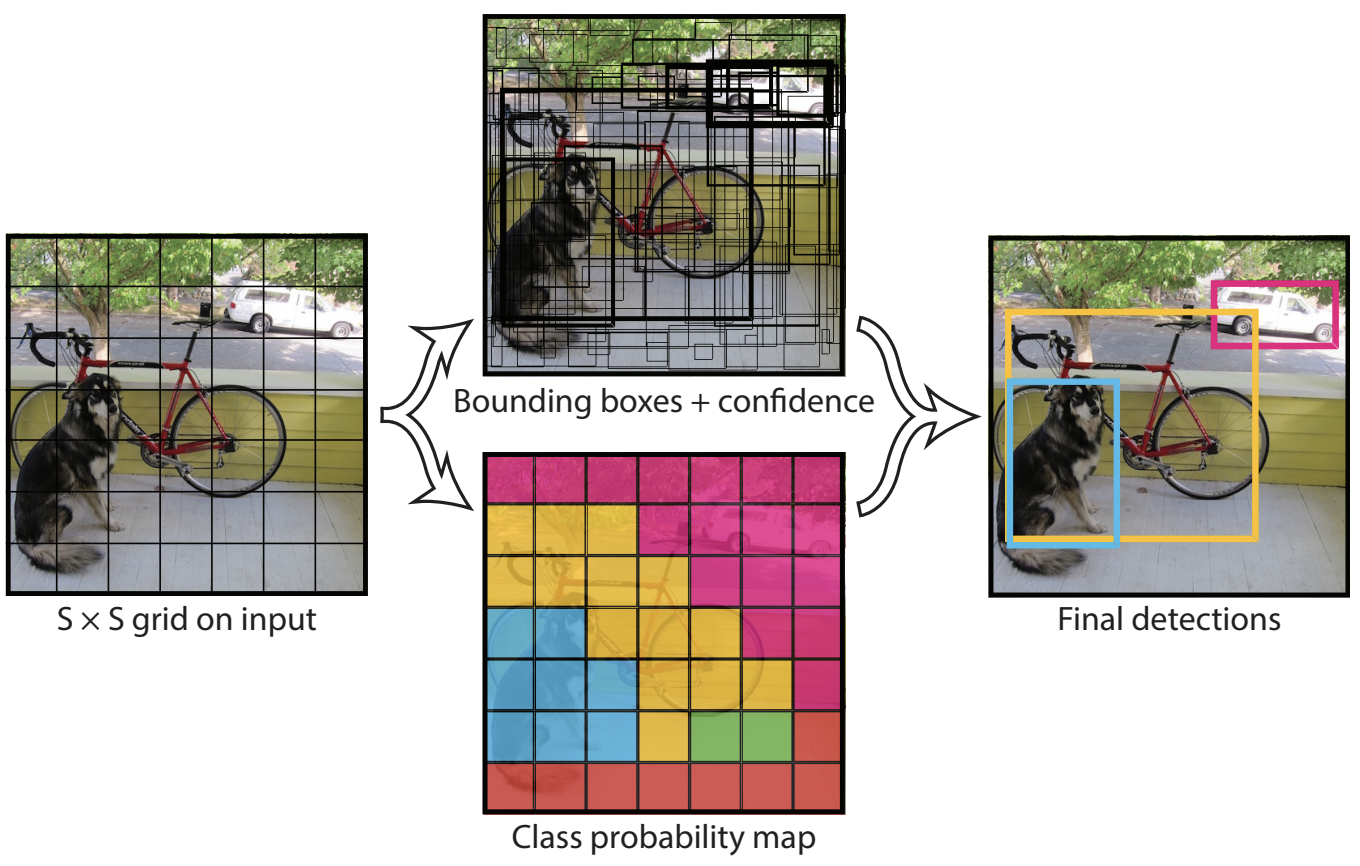
YOLOv1 (2016)
YOLOv1 achieves high speed but has relatively lower detection accuracy compared to two-stage detectors like R-CNN.
- Divides the image into a 7 × 7 grid.
- For each grid cell predicts:
- multiple bounding boxes
(x, y, w, h, confidence) - class probabilities
- multiple bounding boxes
- Each grid cell is responsible for at most one object (the object whose center falls inside the cell)
- Non-Maximum Suppression (NMS) is applied to remove duplicate detections.
YOLOv1 (2016)
YOLOv2 (2017)
YOLOv2 improves YOLOv1 by using a deeper backbone (Darknet-19) and anchor boxes, enabling faster and more accurate single-stage detection over thousands of classes.
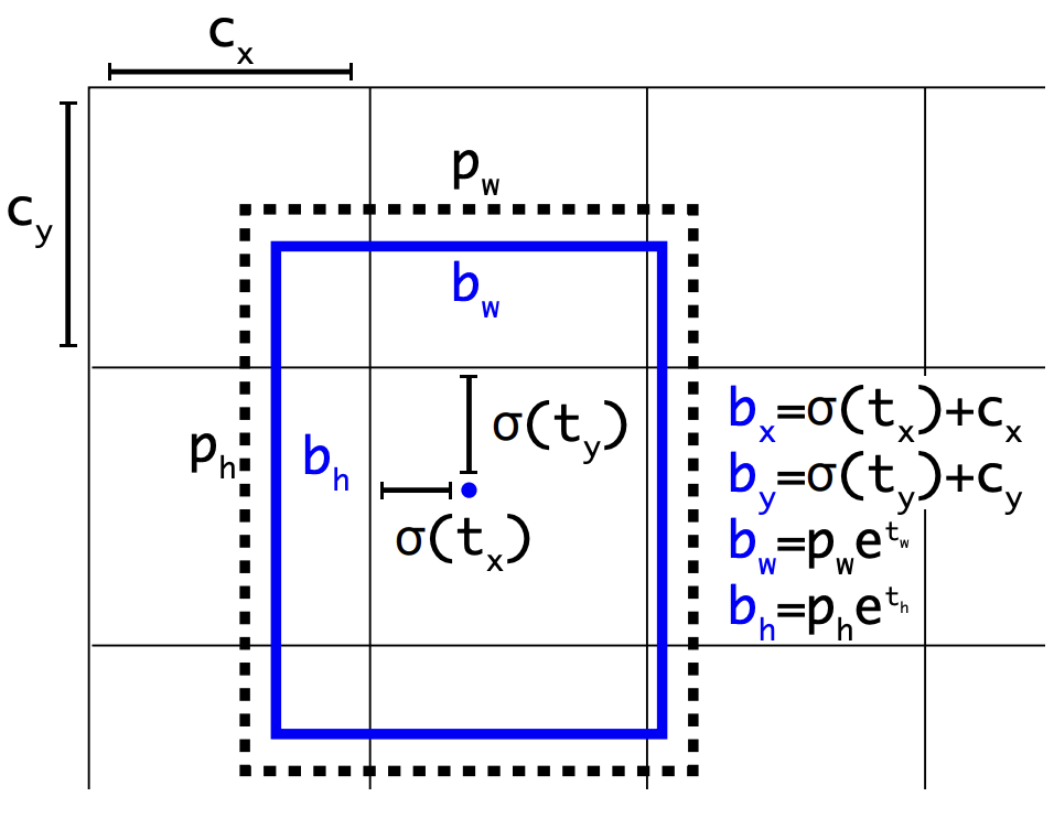
YOLOv2 (2017)
YOLOv2 predicts bounding boxes relative to predefined anchor boxes:
Uses k-means clustering on training data to select anchor box sizes that better match object distributions.
Each grid cell predicts offsets (t_x, t_y, t_w, t_h) for each anchor box (5 in total), which are transformed to final box coordinates:
b_x = \sigma(t_x) + c_x, b_y = \sigma(t_y) + c_y → center relative to the cell
b_w = p_w e^{t_w}, b_h = p_h e^{t_h} → width/height relative to anchor size
Predicts a confidence score for each anchor box (objectness).
Apply NMS.
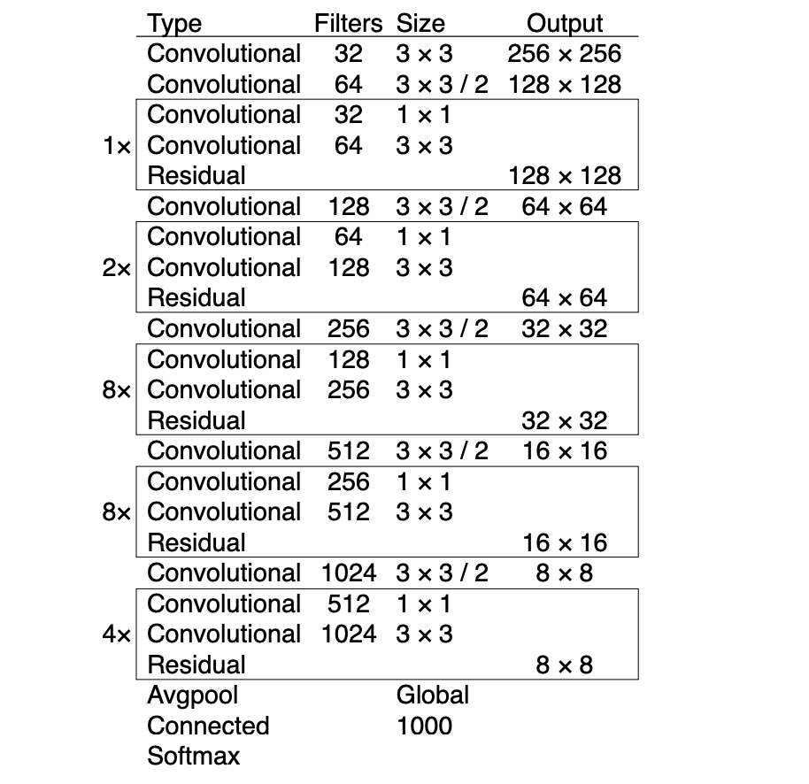
YOLOv3 (2018)
YOLOv3 improves YOLOv2 by using a deeper backbone (Darknet-53) and multi-scale predictions.
YOLOv3 (2018)
Multi-Scale Feature Maps:
- Predictions are made at three scales (e.g., 8×8, 16×16, 32×32).
- Coarse maps detect large objects, fine maps detect small objects.
Anchors per Scale:
- Each scale has its own anchor boxes, selected via k-means clustering for typical object sizes.
Feature Fusion:
- Upsample and concatenate higher-level features with lower-level features to provide context for small objects.
Predictions & Post-Processing:
- Each scale predicts box offsets, objectness, and class probabilities.
- Detections from all scales are merged and filtered with NMS.
YOLOv3 (2018)
After YOLOv3, Joseph Redmon left the field entirely.
If you read his YOLOv3 paper, you can see that he was spending a lot of time on Twitter discussing AI ethics.
The paper itself is written in a casual, almost conversational tone rather than a traditional academic style.
Redmon was deeply concerned about the military applications of his algorithms and the potential privacy risks, such as mass surveillance.
YOLOv3 (2018)
From his YOLOv3 paper:
I guess at least we know the technology is in good hands and definitely won’t be used to harvest your personal information and sell it to…. wait, you’re saying that’s exactly what it will be used for?? Oh.
Well the other people heavily funding vision research are the military and they’ve never done anything horrible like killing lots of people with new technology oh wait…..
But computer vision is already being put to questionable use and as researchers we have a responsibility to at least consider the harm our work might be doing and think of ways to mitigate it. We owe the world that much.
The YOLO branding chaos
After Joseph Redmon left, the YOLO name continued to be used by various researchers, organizations, and companies.
Versions YOLOv4 to YOLOv7 were developed independently, each with their own modifications, training tricks, and implementations.
No central coordination led to confusion:
- Hard to track which version was referenced
- Differences in performance and reliability
- Fragmented naming and forks
Ultralytics YOLOv8 resolved this:
- Built entirely in PyTorch
- Provides a clean, standardized, and accessible framework
- Quickly became the dominant version in practice
YOLO code example
YOLOv8n summary: 129 layers, 3,157,200 parameters, 0 gradients, 8.9 GFLOPs
(129, 3157200, 0, 8.8575488)YOLO(
(model): DetectionModel(
(model): Sequential(
(0): Conv(
(conv): Conv2d(3, 16, kernel_size=(3, 3), stride=(2, 2), padding=(1, 1), bias=False)
(bn): BatchNorm2d(16, eps=0.001, momentum=0.03, affine=True, track_running_stats=True)
(act): SiLU(inplace=True)
)
(1): Conv(
(conv): Conv2d(16, 32, kernel_size=(3, 3), stride=(2, 2), padding=(1, 1), bias=False)
(bn): BatchNorm2d(32, eps=0.001, momentum=0.03, affine=True, track_running_stats=True)
(act): SiLU(inplace=True)
)
(2): C2f(
(cv1): Conv(
(conv): Conv2d(32, 32, kernel_size=(1, 1), stride=(1, 1), bias=False)
(bn): BatchNorm2d(32, eps=0.001, momentum=0.03, affine=True, track_running_stats=True)
(act): SiLU(inplace=True)
)
(cv2): Conv(
(conv): Conv2d(48, 32, kernel_size=(1, 1), stride=(1, 1), bias=False)
(bn): BatchNorm2d(32, eps=0.001, momentum=0.03, affine=True, track_running_stats=True)
(act): SiLU(inplace=True)
)
(m): ModuleList(
(0): Bottleneck(
(cv1): Conv(
(conv): Conv2d(16, 16, kernel_size=(3, 3), stride=(1, 1), padding=(1, 1), bias=False)
(bn): BatchNorm2d(16, eps=0.001, momentum=0.03, affine=True, track_running_stats=True)
(act): SiLU(inplace=True)
)
(cv2): Conv(
(conv): Conv2d(16, 16, kernel_size=(3, 3), stride=(1, 1), padding=(1, 1), bias=False)
(bn): BatchNorm2d(16, eps=0.001, momentum=0.03, affine=True, track_running_stats=True)
(act): SiLU(inplace=True)
)
)
)
)
(3): Conv(
(conv): Conv2d(32, 64, kernel_size=(3, 3), stride=(2, 2), padding=(1, 1), bias=False)
(bn): BatchNorm2d(64, eps=0.001, momentum=0.03, affine=True, track_running_stats=True)
(act): SiLU(inplace=True)
)
(4): C2f(
(cv1): Conv(
(conv): Conv2d(64, 64, kernel_size=(1, 1), stride=(1, 1), bias=False)
(bn): BatchNorm2d(64, eps=0.001, momentum=0.03, affine=True, track_running_stats=True)
(act): SiLU(inplace=True)
)
(cv2): Conv(
(conv): Conv2d(128, 64, kernel_size=(1, 1), stride=(1, 1), bias=False)
(bn): BatchNorm2d(64, eps=0.001, momentum=0.03, affine=True, track_running_stats=True)
(act): SiLU(inplace=True)
)
(m): ModuleList(
(0-1): 2 x Bottleneck(
(cv1): Conv(
(conv): Conv2d(32, 32, kernel_size=(3, 3), stride=(1, 1), padding=(1, 1), bias=False)
(bn): BatchNorm2d(32, eps=0.001, momentum=0.03, affine=True, track_running_stats=True)
(act): SiLU(inplace=True)
)
(cv2): Conv(
(conv): Conv2d(32, 32, kernel_size=(3, 3), stride=(1, 1), padding=(1, 1), bias=False)
(bn): BatchNorm2d(32, eps=0.001, momentum=0.03, affine=True, track_running_stats=True)
(act): SiLU(inplace=True)
)
)
)
)
(5): Conv(
(conv): Conv2d(64, 128, kernel_size=(3, 3), stride=(2, 2), padding=(1, 1), bias=False)
(bn): BatchNorm2d(128, eps=0.001, momentum=0.03, affine=True, track_running_stats=True)
(act): SiLU(inplace=True)
)
(6): C2f(
(cv1): Conv(
(conv): Conv2d(128, 128, kernel_size=(1, 1), stride=(1, 1), bias=False)
(bn): BatchNorm2d(128, eps=0.001, momentum=0.03, affine=True, track_running_stats=True)
(act): SiLU(inplace=True)
)
(cv2): Conv(
(conv): Conv2d(256, 128, kernel_size=(1, 1), stride=(1, 1), bias=False)
(bn): BatchNorm2d(128, eps=0.001, momentum=0.03, affine=True, track_running_stats=True)
(act): SiLU(inplace=True)
)
(m): ModuleList(
(0-1): 2 x Bottleneck(
(cv1): Conv(
(conv): Conv2d(64, 64, kernel_size=(3, 3), stride=(1, 1), padding=(1, 1), bias=False)
(bn): BatchNorm2d(64, eps=0.001, momentum=0.03, affine=True, track_running_stats=True)
(act): SiLU(inplace=True)
)
(cv2): Conv(
(conv): Conv2d(64, 64, kernel_size=(3, 3), stride=(1, 1), padding=(1, 1), bias=False)
(bn): BatchNorm2d(64, eps=0.001, momentum=0.03, affine=True, track_running_stats=True)
(act): SiLU(inplace=True)
)
)
)
)
(7): Conv(
(conv): Conv2d(128, 256, kernel_size=(3, 3), stride=(2, 2), padding=(1, 1), bias=False)
(bn): BatchNorm2d(256, eps=0.001, momentum=0.03, affine=True, track_running_stats=True)
(act): SiLU(inplace=True)
)
(8): C2f(
(cv1): Conv(
(conv): Conv2d(256, 256, kernel_size=(1, 1), stride=(1, 1), bias=False)
(bn): BatchNorm2d(256, eps=0.001, momentum=0.03, affine=True, track_running_stats=True)
(act): SiLU(inplace=True)
)
(cv2): Conv(
(conv): Conv2d(384, 256, kernel_size=(1, 1), stride=(1, 1), bias=False)
(bn): BatchNorm2d(256, eps=0.001, momentum=0.03, affine=True, track_running_stats=True)
(act): SiLU(inplace=True)
)
(m): ModuleList(
(0): Bottleneck(
(cv1): Conv(
(conv): Conv2d(128, 128, kernel_size=(3, 3), stride=(1, 1), padding=(1, 1), bias=False)
(bn): BatchNorm2d(128, eps=0.001, momentum=0.03, affine=True, track_running_stats=True)
(act): SiLU(inplace=True)
)
(cv2): Conv(
(conv): Conv2d(128, 128, kernel_size=(3, 3), stride=(1, 1), padding=(1, 1), bias=False)
(bn): BatchNorm2d(128, eps=0.001, momentum=0.03, affine=True, track_running_stats=True)
(act): SiLU(inplace=True)
)
)
)
)
(9): SPPF(
(cv1): Conv(
(conv): Conv2d(256, 128, kernel_size=(1, 1), stride=(1, 1), bias=False)
(bn): BatchNorm2d(128, eps=0.001, momentum=0.03, affine=True, track_running_stats=True)
(act): SiLU(inplace=True)
)
(cv2): Conv(
(conv): Conv2d(512, 256, kernel_size=(1, 1), stride=(1, 1), bias=False)
(bn): BatchNorm2d(256, eps=0.001, momentum=0.03, affine=True, track_running_stats=True)
(act): SiLU(inplace=True)
)
(m): MaxPool2d(kernel_size=5, stride=1, padding=2, dilation=1, ceil_mode=False)
)
(10): Upsample(scale_factor=2.0, mode='nearest')
(11): Concat()
(12): C2f(
(cv1): Conv(
(conv): Conv2d(384, 128, kernel_size=(1, 1), stride=(1, 1), bias=False)
(bn): BatchNorm2d(128, eps=0.001, momentum=0.03, affine=True, track_running_stats=True)
(act): SiLU(inplace=True)
)
(cv2): Conv(
(conv): Conv2d(192, 128, kernel_size=(1, 1), stride=(1, 1), bias=False)
(bn): BatchNorm2d(128, eps=0.001, momentum=0.03, affine=True, track_running_stats=True)
(act): SiLU(inplace=True)
)
(m): ModuleList(
(0): Bottleneck(
(cv1): Conv(
(conv): Conv2d(64, 64, kernel_size=(3, 3), stride=(1, 1), padding=(1, 1), bias=False)
(bn): BatchNorm2d(64, eps=0.001, momentum=0.03, affine=True, track_running_stats=True)
(act): SiLU(inplace=True)
)
(cv2): Conv(
(conv): Conv2d(64, 64, kernel_size=(3, 3), stride=(1, 1), padding=(1, 1), bias=False)
(bn): BatchNorm2d(64, eps=0.001, momentum=0.03, affine=True, track_running_stats=True)
(act): SiLU(inplace=True)
)
)
)
)
(13): Upsample(scale_factor=2.0, mode='nearest')
(14): Concat()
(15): C2f(
(cv1): Conv(
(conv): Conv2d(192, 64, kernel_size=(1, 1), stride=(1, 1), bias=False)
(bn): BatchNorm2d(64, eps=0.001, momentum=0.03, affine=True, track_running_stats=True)
(act): SiLU(inplace=True)
)
(cv2): Conv(
(conv): Conv2d(96, 64, kernel_size=(1, 1), stride=(1, 1), bias=False)
(bn): BatchNorm2d(64, eps=0.001, momentum=0.03, affine=True, track_running_stats=True)
(act): SiLU(inplace=True)
)
(m): ModuleList(
(0): Bottleneck(
(cv1): Conv(
(conv): Conv2d(32, 32, kernel_size=(3, 3), stride=(1, 1), padding=(1, 1), bias=False)
(bn): BatchNorm2d(32, eps=0.001, momentum=0.03, affine=True, track_running_stats=True)
(act): SiLU(inplace=True)
)
(cv2): Conv(
(conv): Conv2d(32, 32, kernel_size=(3, 3), stride=(1, 1), padding=(1, 1), bias=False)
(bn): BatchNorm2d(32, eps=0.001, momentum=0.03, affine=True, track_running_stats=True)
(act): SiLU(inplace=True)
)
)
)
)
(16): Conv(
(conv): Conv2d(64, 64, kernel_size=(3, 3), stride=(2, 2), padding=(1, 1), bias=False)
(bn): BatchNorm2d(64, eps=0.001, momentum=0.03, affine=True, track_running_stats=True)
(act): SiLU(inplace=True)
)
(17): Concat()
(18): C2f(
(cv1): Conv(
(conv): Conv2d(192, 128, kernel_size=(1, 1), stride=(1, 1), bias=False)
(bn): BatchNorm2d(128, eps=0.001, momentum=0.03, affine=True, track_running_stats=True)
(act): SiLU(inplace=True)
)
(cv2): Conv(
(conv): Conv2d(192, 128, kernel_size=(1, 1), stride=(1, 1), bias=False)
(bn): BatchNorm2d(128, eps=0.001, momentum=0.03, affine=True, track_running_stats=True)
(act): SiLU(inplace=True)
)
(m): ModuleList(
(0): Bottleneck(
(cv1): Conv(
(conv): Conv2d(64, 64, kernel_size=(3, 3), stride=(1, 1), padding=(1, 1), bias=False)
(bn): BatchNorm2d(64, eps=0.001, momentum=0.03, affine=True, track_running_stats=True)
(act): SiLU(inplace=True)
)
(cv2): Conv(
(conv): Conv2d(64, 64, kernel_size=(3, 3), stride=(1, 1), padding=(1, 1), bias=False)
(bn): BatchNorm2d(64, eps=0.001, momentum=0.03, affine=True, track_running_stats=True)
(act): SiLU(inplace=True)
)
)
)
)
(19): Conv(
(conv): Conv2d(128, 128, kernel_size=(3, 3), stride=(2, 2), padding=(1, 1), bias=False)
(bn): BatchNorm2d(128, eps=0.001, momentum=0.03, affine=True, track_running_stats=True)
(act): SiLU(inplace=True)
)
(20): Concat()
(21): C2f(
(cv1): Conv(
(conv): Conv2d(384, 256, kernel_size=(1, 1), stride=(1, 1), bias=False)
(bn): BatchNorm2d(256, eps=0.001, momentum=0.03, affine=True, track_running_stats=True)
(act): SiLU(inplace=True)
)
(cv2): Conv(
(conv): Conv2d(384, 256, kernel_size=(1, 1), stride=(1, 1), bias=False)
(bn): BatchNorm2d(256, eps=0.001, momentum=0.03, affine=True, track_running_stats=True)
(act): SiLU(inplace=True)
)
(m): ModuleList(
(0): Bottleneck(
(cv1): Conv(
(conv): Conv2d(128, 128, kernel_size=(3, 3), stride=(1, 1), padding=(1, 1), bias=False)
(bn): BatchNorm2d(128, eps=0.001, momentum=0.03, affine=True, track_running_stats=True)
(act): SiLU(inplace=True)
)
(cv2): Conv(
(conv): Conv2d(128, 128, kernel_size=(3, 3), stride=(1, 1), padding=(1, 1), bias=False)
(bn): BatchNorm2d(128, eps=0.001, momentum=0.03, affine=True, track_running_stats=True)
(act): SiLU(inplace=True)
)
)
)
)
(22): Detect(
(cv2): ModuleList(
(0): Sequential(
(0): Conv(
(conv): Conv2d(64, 64, kernel_size=(3, 3), stride=(1, 1), padding=(1, 1), bias=False)
(bn): BatchNorm2d(64, eps=0.001, momentum=0.03, affine=True, track_running_stats=True)
(act): SiLU(inplace=True)
)
(1): Conv(
(conv): Conv2d(64, 64, kernel_size=(3, 3), stride=(1, 1), padding=(1, 1), bias=False)
(bn): BatchNorm2d(64, eps=0.001, momentum=0.03, affine=True, track_running_stats=True)
(act): SiLU(inplace=True)
)
(2): Conv2d(64, 64, kernel_size=(1, 1), stride=(1, 1))
)
(1): Sequential(
(0): Conv(
(conv): Conv2d(128, 64, kernel_size=(3, 3), stride=(1, 1), padding=(1, 1), bias=False)
(bn): BatchNorm2d(64, eps=0.001, momentum=0.03, affine=True, track_running_stats=True)
(act): SiLU(inplace=True)
)
(1): Conv(
(conv): Conv2d(64, 64, kernel_size=(3, 3), stride=(1, 1), padding=(1, 1), bias=False)
(bn): BatchNorm2d(64, eps=0.001, momentum=0.03, affine=True, track_running_stats=True)
(act): SiLU(inplace=True)
)
(2): Conv2d(64, 64, kernel_size=(1, 1), stride=(1, 1))
)
(2): Sequential(
(0): Conv(
(conv): Conv2d(256, 64, kernel_size=(3, 3), stride=(1, 1), padding=(1, 1), bias=False)
(bn): BatchNorm2d(64, eps=0.001, momentum=0.03, affine=True, track_running_stats=True)
(act): SiLU(inplace=True)
)
(1): Conv(
(conv): Conv2d(64, 64, kernel_size=(3, 3), stride=(1, 1), padding=(1, 1), bias=False)
(bn): BatchNorm2d(64, eps=0.001, momentum=0.03, affine=True, track_running_stats=True)
(act): SiLU(inplace=True)
)
(2): Conv2d(64, 64, kernel_size=(1, 1), stride=(1, 1))
)
)
(cv3): ModuleList(
(0): Sequential(
(0): Conv(
(conv): Conv2d(64, 80, kernel_size=(3, 3), stride=(1, 1), padding=(1, 1), bias=False)
(bn): BatchNorm2d(80, eps=0.001, momentum=0.03, affine=True, track_running_stats=True)
(act): SiLU(inplace=True)
)
(1): Conv(
(conv): Conv2d(80, 80, kernel_size=(3, 3), stride=(1, 1), padding=(1, 1), bias=False)
(bn): BatchNorm2d(80, eps=0.001, momentum=0.03, affine=True, track_running_stats=True)
(act): SiLU(inplace=True)
)
(2): Conv2d(80, 80, kernel_size=(1, 1), stride=(1, 1))
)
(1): Sequential(
(0): Conv(
(conv): Conv2d(128, 80, kernel_size=(3, 3), stride=(1, 1), padding=(1, 1), bias=False)
(bn): BatchNorm2d(80, eps=0.001, momentum=0.03, affine=True, track_running_stats=True)
(act): SiLU(inplace=True)
)
(1): Conv(
(conv): Conv2d(80, 80, kernel_size=(3, 3), stride=(1, 1), padding=(1, 1), bias=False)
(bn): BatchNorm2d(80, eps=0.001, momentum=0.03, affine=True, track_running_stats=True)
(act): SiLU(inplace=True)
)
(2): Conv2d(80, 80, kernel_size=(1, 1), stride=(1, 1))
)
(2): Sequential(
(0): Conv(
(conv): Conv2d(256, 80, kernel_size=(3, 3), stride=(1, 1), padding=(1, 1), bias=False)
(bn): BatchNorm2d(80, eps=0.001, momentum=0.03, affine=True, track_running_stats=True)
(act): SiLU(inplace=True)
)
(1): Conv(
(conv): Conv2d(80, 80, kernel_size=(3, 3), stride=(1, 1), padding=(1, 1), bias=False)
(bn): BatchNorm2d(80, eps=0.001, momentum=0.03, affine=True, track_running_stats=True)
(act): SiLU(inplace=True)
)
(2): Conv2d(80, 80, kernel_size=(1, 1), stride=(1, 1))
)
)
(dfl): DFL(
(conv): Conv2d(16, 1, kernel_size=(1, 1), stride=(1, 1), bias=False)
)
)
)
)
)
signature: (
source: 'str | Path | int | Image.Image | list | tuple | np.ndarray | torch.Tensor' = None,
stream: 'bool' = False,
**kwargs: 'Any'
) -> 'list'YOLO prediction
image 1/1 /Users/patrickli/Desktop/rproj/ibsar-cv-workshop/instructor/slides/slide_figures/original.png: 640x448 1 cat, 27.7ms
Speed: 1.0ms preprocess, 27.7ms inference, 0.6ms postprocess per image at shape (1, 3, 640, 448)'slide_figures/cat_object_detect.png'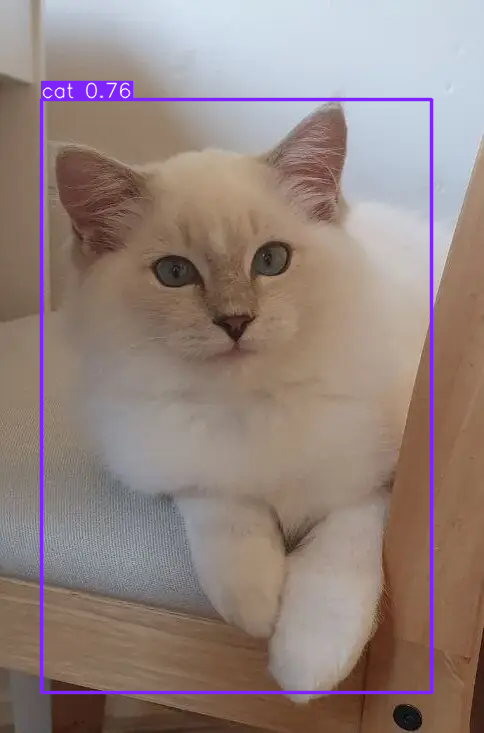
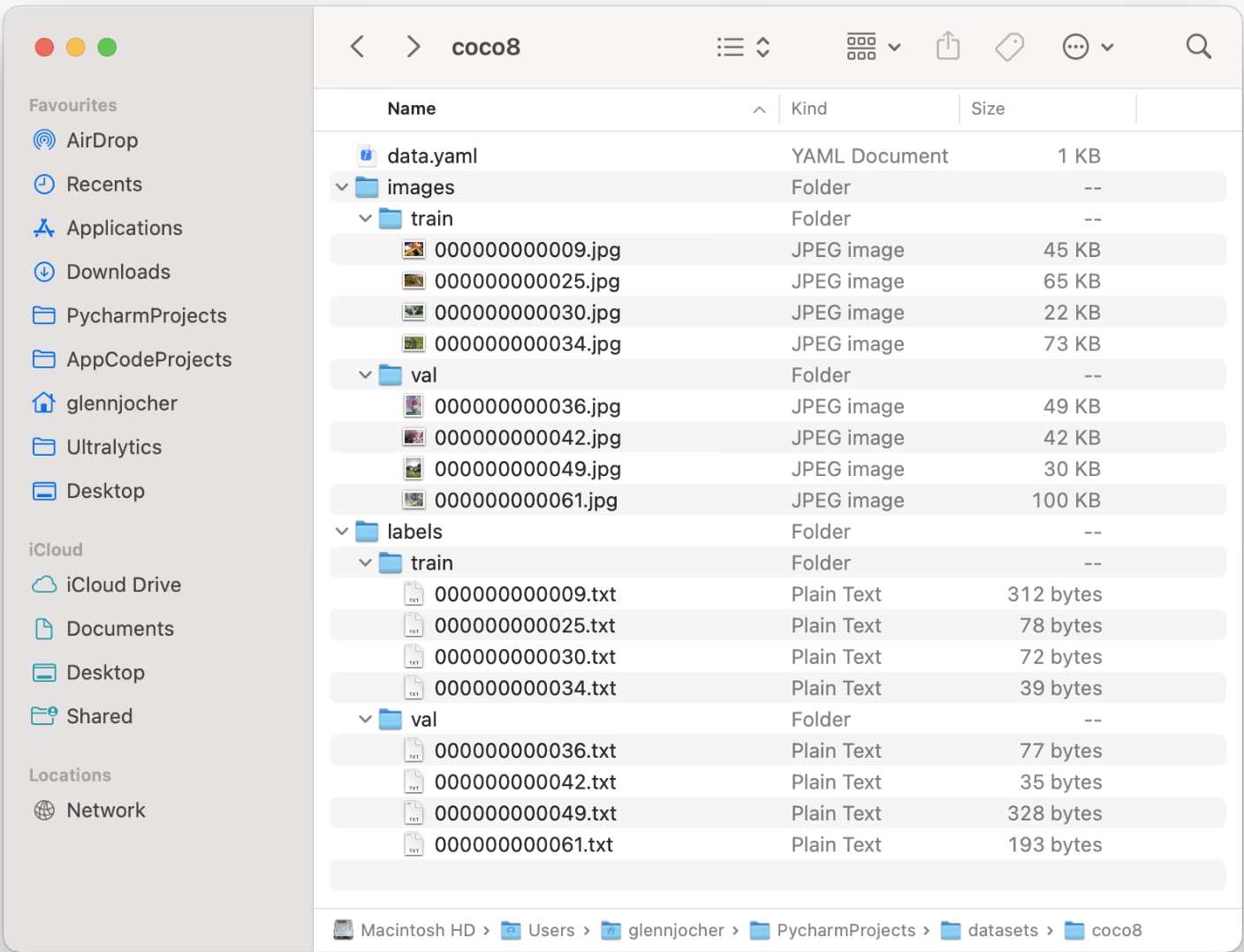
YOLO training config file (data.yaml)
data.yaml:
# Ultralytics 🚀 AGPL-3.0 License - https://ultralytics.com/license

# COCO8 dataset (first 8 images from COCO train2017) by Ultralytics
# Documentation: https://docs.ultralytics.com/datasets/detect/coco8/
# Example usage: yolo train data=coco8.yaml
# parent
# ├── ultralytics
# └── datasets
#     └── coco8 ← downloads here (1 MB)

# Train/val/test sets as 1) dir: path/to/imgs, 2) file: path/to/imgs.txt, or 3) list: [path/to/imgs1, path/to/imgs2, ..]
path: coco8 # dataset root dir
train: images/train # train images (relative to 'path') 4 images
val: images/val # val images (relative to 'path') 4 images
test: # test images (optional)

# Classes
names:
  0: person
  1: bicycle
  2: car
  3: motorcycle
  4: airplane
  5: bus
  6: train
  7: truck
  8: boat
  9: traffic light
  10: fire hydrant
  11: stop sign
  12: parking meter
  13: bench
  14: bird
  15: cat
  16: dog
  17: horse
  18: sheep
  19: cow
  20: elephant
  21: bear
  22: zebra
  23: giraffe
  24: backpack
  25: umbrella
  26: handbag
  27: tie
  28: suitcase
  29: frisbee
  30: skis
  31: snowboard
  32: sports ball
  33: kite
  34: baseball bat
  35: baseball glove
  36: skateboard
  37: surfboard
  38: tennis racket
  39: bottle
  40: wine glass
  41: cup
  42: fork
  43: knife
  44: spoon
  45: bowl
  46: banana
  47: apple
  48: sandwich
  49: orange
  50: broccoli
  51: carrot
  52: hot dog
  53: pizza
  54: donut
  55: cake
  56: chair
  57: couch
  58: potted plant
  59: bed
  60: dining table
  61: toilet
  62: tv
  63: laptop
  64: mouse
  65: remote
  66: keyboard
  67: cell phone
  68: microwave
  69: oven
  70: toaster
  71: sink
  72: refrigerator
  73: book
  74: clock
  75: vase
  76: scissors
  77: teddy bear
  78: hair drier
  79: toothbrush

# Download script/URL (optional)
download: https://github.com/ultralytics/assets/releases/download/v0.0.0/coco8.zip
YOLO training
model$train(
    data = 'data.yaml',   # dataset config (train/val paths + class names)
    epochs = 100L,        # number of epochs
    imgsz = 640L,         # image size (square)
    batch = 16L,          # batch size
    lr0 = 0.01,           # inital learning rate
    optimizer = 'auto',   # optimizer: e.g. 'SGD', 'Adam'
    device = NULL,        # device: 'cpu', '0', '0,1', etc.
    workers = 8L,         # dataloader workers
    project = 'runs/train', # save path
    name = 'exp',         # folder name
    exist_ok = FALSE,     # overwrite existing folder
    pretrained = TRUE,    # use pretrained weights if True
    patience = 50L,       # early stopping patience
    save = TRUE,          # save final model
    save_period = 10L,    # save every N epochs (-1 = disabled)
    seed = 0,             # random seed
    verbose = TRUE,       # print progress
)
YOLO live camera demo
Camera Capture:
- A webcam (built-in or external) provides live video frames.
- OpenCV (
cv2.VideoCapture) continuously reads frames from the camera.
Object Detection: YOLO predicts the objects in the frame, providing class labels and bounding boxes.
Display: Bounding boxes and labels are drawn on the frame by OpenCV in real time.
Exercises 4

Slides URL: https://ibsar-cv-workshop.patrickli.org/ | Canberra time