model <- keras$Model(vgg16$input,
vgg16$get_layer("flatten")$output)
final_conv_pred <- haku |>
keras$layers$Resizing(224L, 224L)() |>
torch$unsqueeze(0L) |>
keras$applications$vgg16$preprocess_input() |>
model$predict()
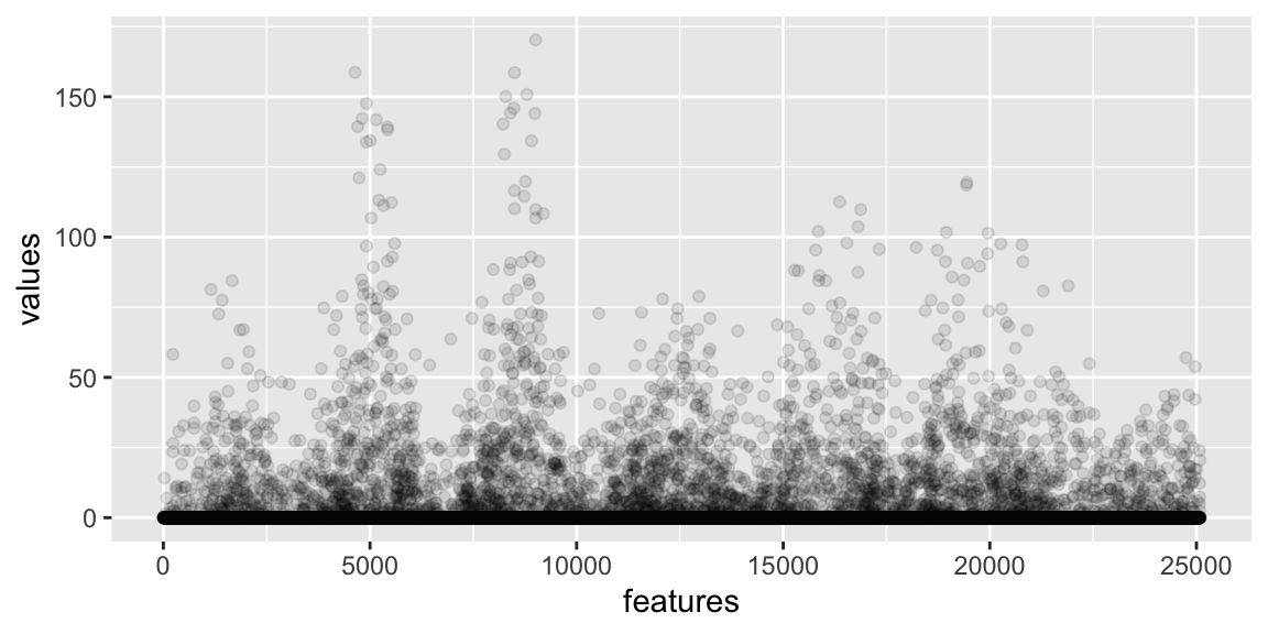
data.frame(features = 1:25088,
values = py_to_r(final_conv_pred[0])) |>
ggplot() +
geom_point(aes(features, values), alpha = 0.1)CNN model interpretation
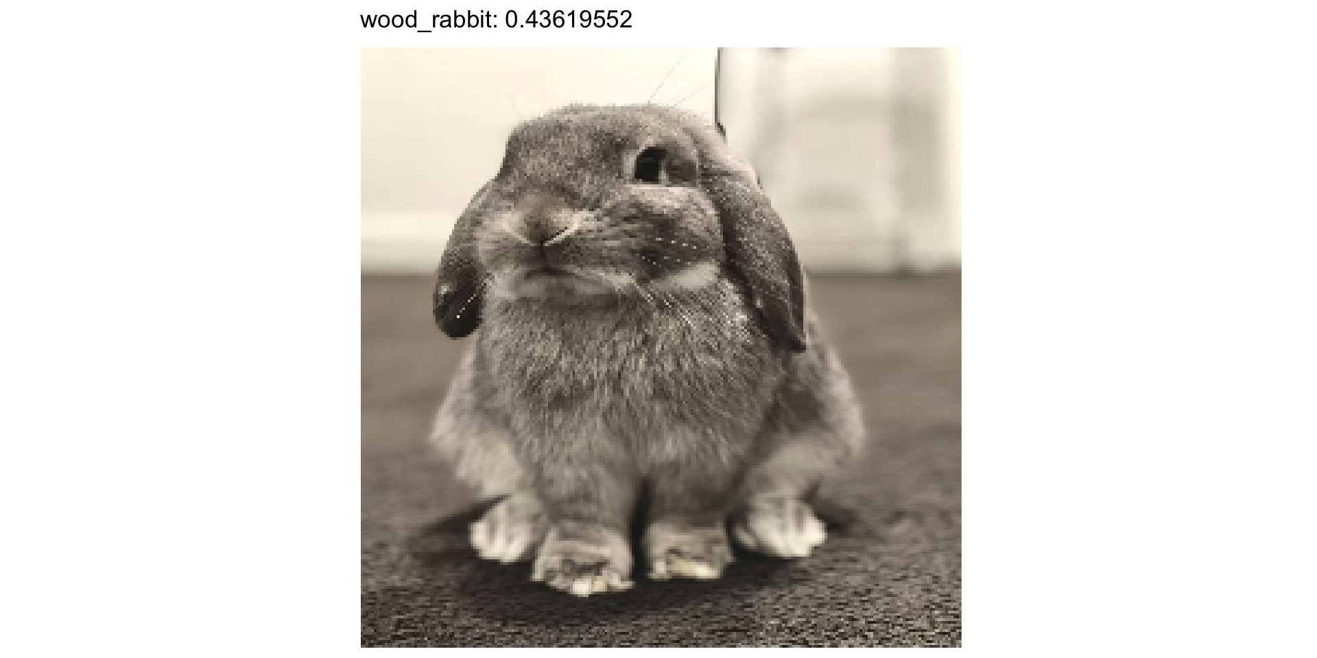
block1_conv1 in VGG16
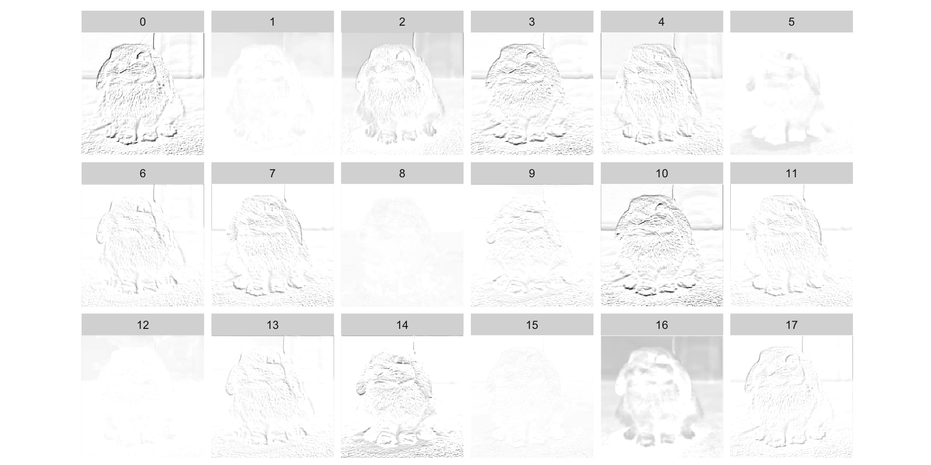
block2_conv1 in VGG16
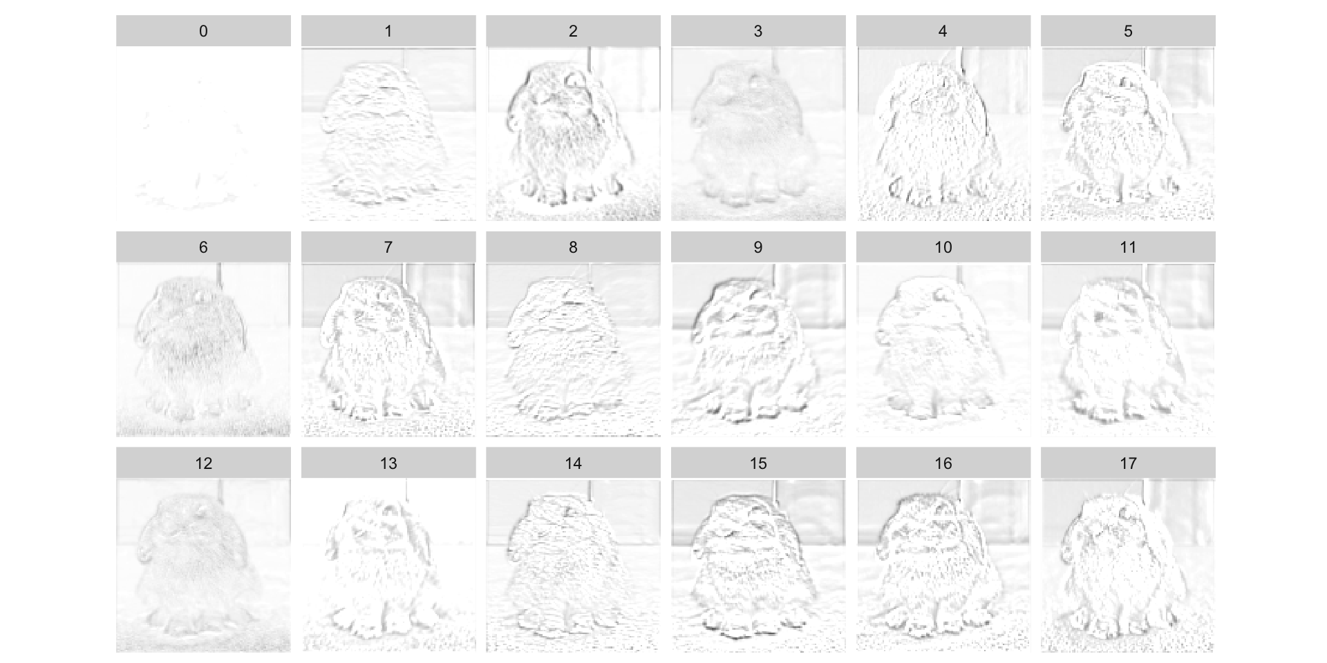
block3_conv1 in VGG16
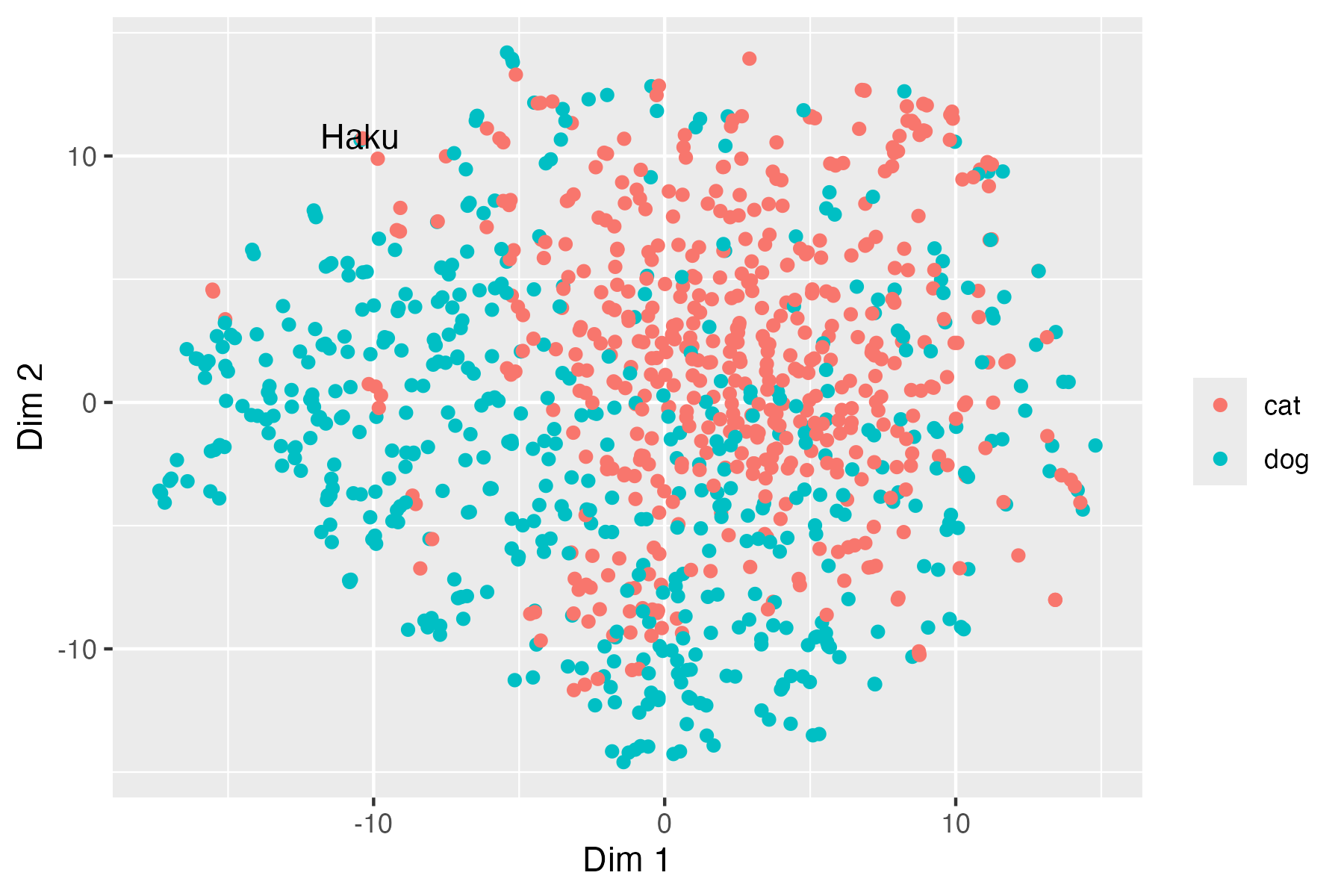
Embedding space
Outputs from the final convolutional block capture hierarchical visual features, mapping similar images close together and dissimilar ones farther apart.
Embeddings can be visualized or used for tasks such as retrieval, classification, and clustering.
Visualize the embedding with t-SNE
Significant Overlap: Cat and dog embeddings mix heavily, indicating weak class separation and substantial sharing of visual features in VGG16’s feature space.
Partial Clustering: Cats tend to group toward the right/upper region.
Haku’s Position: Haku sits at the boundary of both classes, suggesting it is distinct from both classes yet still partially resemble visual aspects of cats and dogs.
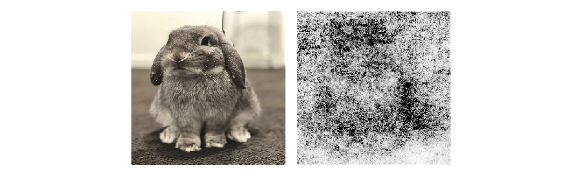
Vanilla gradient
They are often noisy and work best on simpler, task-specific models.
Grad-CAM
- Target layer: Pick a late convolutional layer with good spatial and semantic info.
- Activations: Record feature maps from the forward pass.
- Gradients: Backpropagate the class score to the feature maps.
- Pooling: Average gradients spatially to get channel weights.
- Combine: Weight feature maps and sum to form the heatmap.
- ReLU: Keep only positive contributions.
- Normalize: Scale to 0–1 and resize to input dimensions.
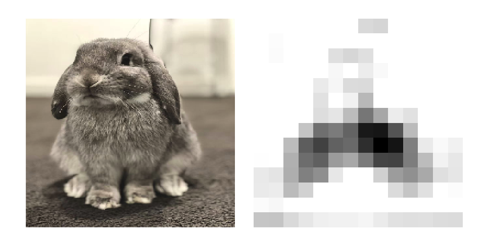
first_part <- keras$Model(vgg16$input,
                          vgg16$get_layer("block5_conv3")$output)
second_part <- keras$Model(vgg16$get_layer("block5_pool")$input,
                           vgg16$output)

resized <- haku |>
  keras$layers$Resizing(224L, 224L)() |>
  torch$unsqueeze(0L)
invisible(resized$requires_grad_())
first_pred <- resized |>
  keras$applications$vgg16$preprocess_input() |>
  first_part()

second_pred <- first_pred |>
  second_part()
grad <- torch$autograd$grad(second_pred[0][330], first_pred)[0][0]

positive_map <- (grad$mean(dim = tuple(0L, 1L))$view(1L, 1L, 512L) * first_pred[0])$sum(dim = 2L) |>
  keras$layers$ReLU()()

positive_map <- (positive_map - positive_map$min()) / (positive_map$max() - positive_map$min())
positive_map <- 1 - positive_map

p1 <- resized[0]$detach()$cpu()$numpy() |>
  plot_rgb(axis = FALSE)
p2 <- positive_map$unsqueeze(-1L)$`repeat`(1L, 1L, 3L)$detach()$cpu()$numpy() |>
  plot_rgb(max_value = 1, axis = FALSE)
patchwork::wrap_plots(p1, p2, ncol = 1)Self-supervised learning
- No labels required during pretraining.
- Pretext tasks teach the network useful features (e.g., predicting missing image patches, rotations, or contrastive similarity). We then fine-tune the learned representations for classification.
\overset{\text{Predict}}{\Longrightarrow}

Exercises 3
Select the best-performing NN and CNN models we have trained so far. Then, for training image No.2, visualize their raw gradients. In addition, generate a Grad-CAM visualization for the CNN model.