Why fully-connected NN struggle?
- No translation invariance: the same object in a different place looks completely different.
array([[0.4848306 , 0.51516944]], dtype=float32)array([[0.7504414 , 0.24955861]], dtype=float32)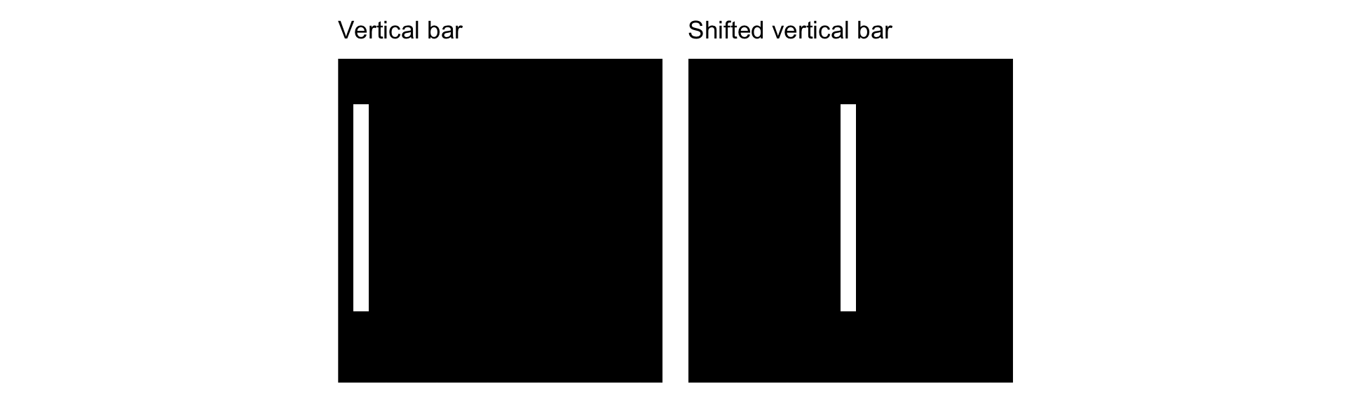
Why fully-connected NN struggle?
- Ignored input topology: the spatial structure of images and local correlations are not inherently utilized.
Convolutional neural networks
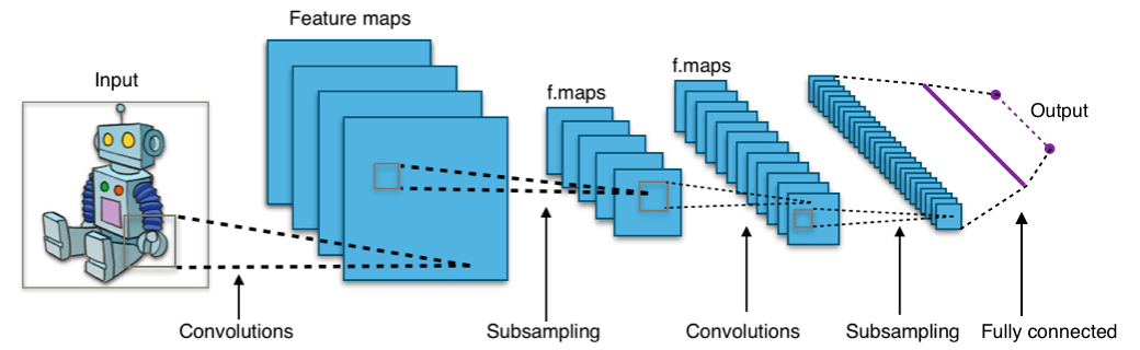
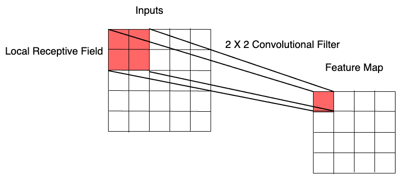
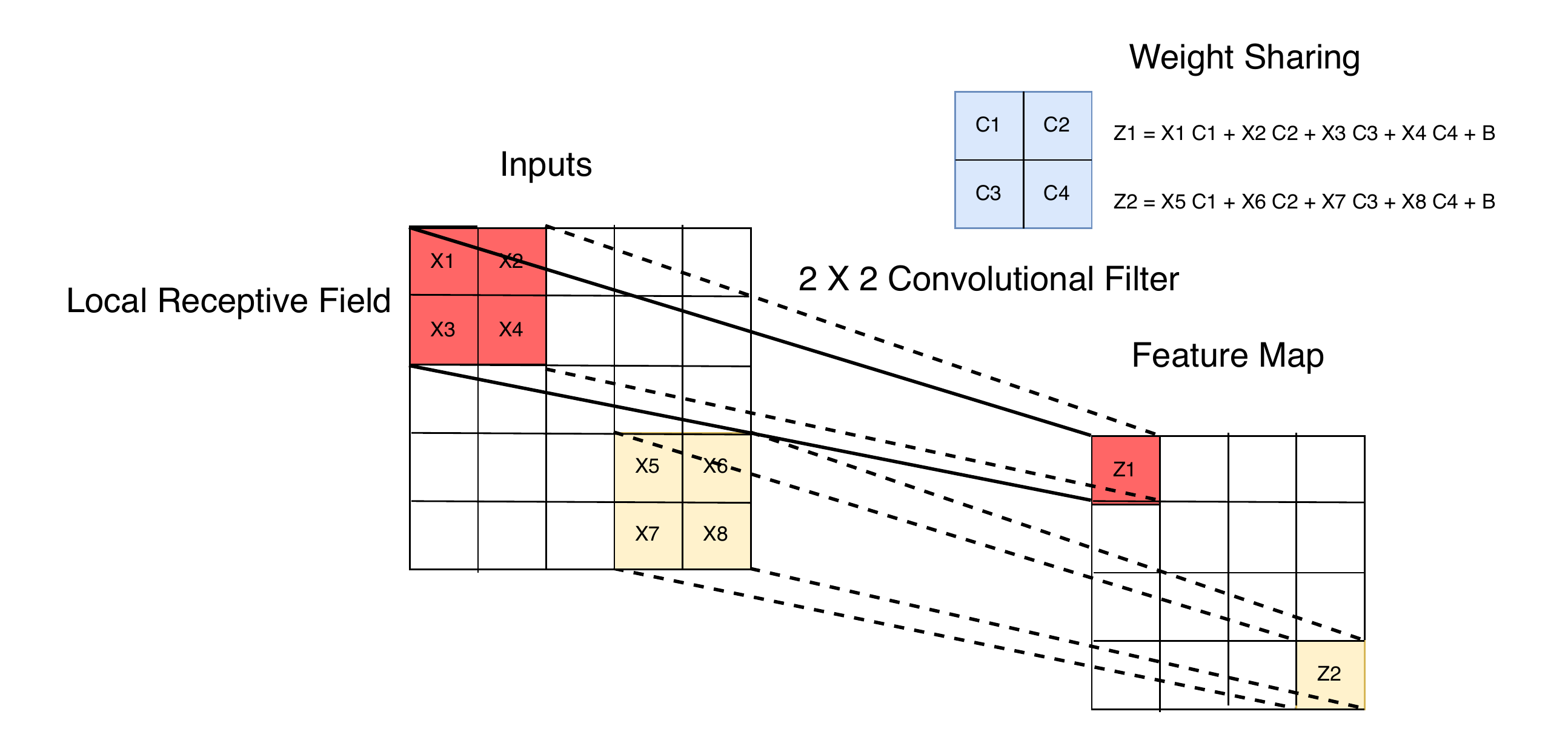
Local receptive fields
Local receptive fields extract basic features (e.g. edges, corners), which are combined in deeper layers to detect higher order patterns.
Weight sharing
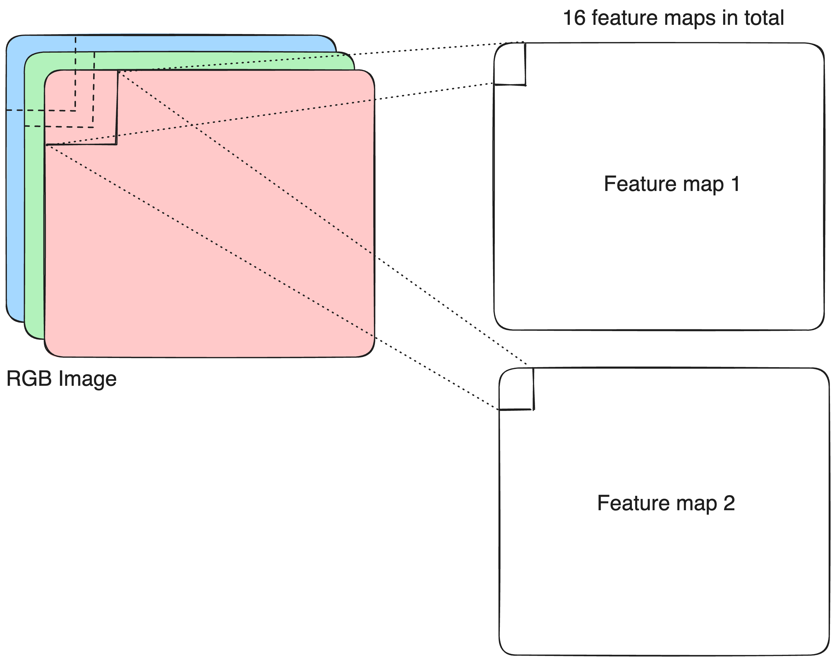
Conv2D layer
filtersspecifies the number of convolutional filters (feature maps).
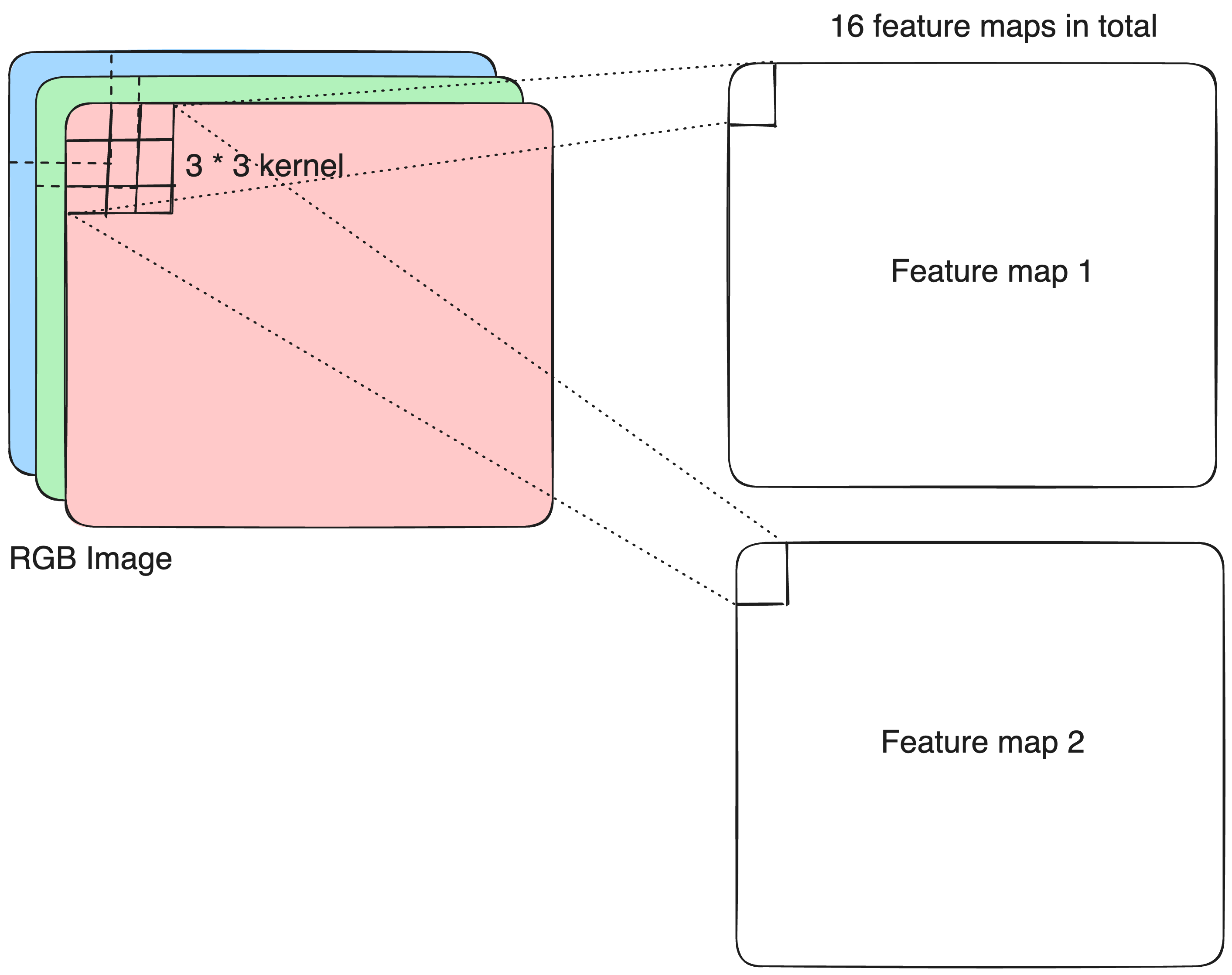
Conv2D layer
kernel_sizedefines the height and width of each convolutional filter.
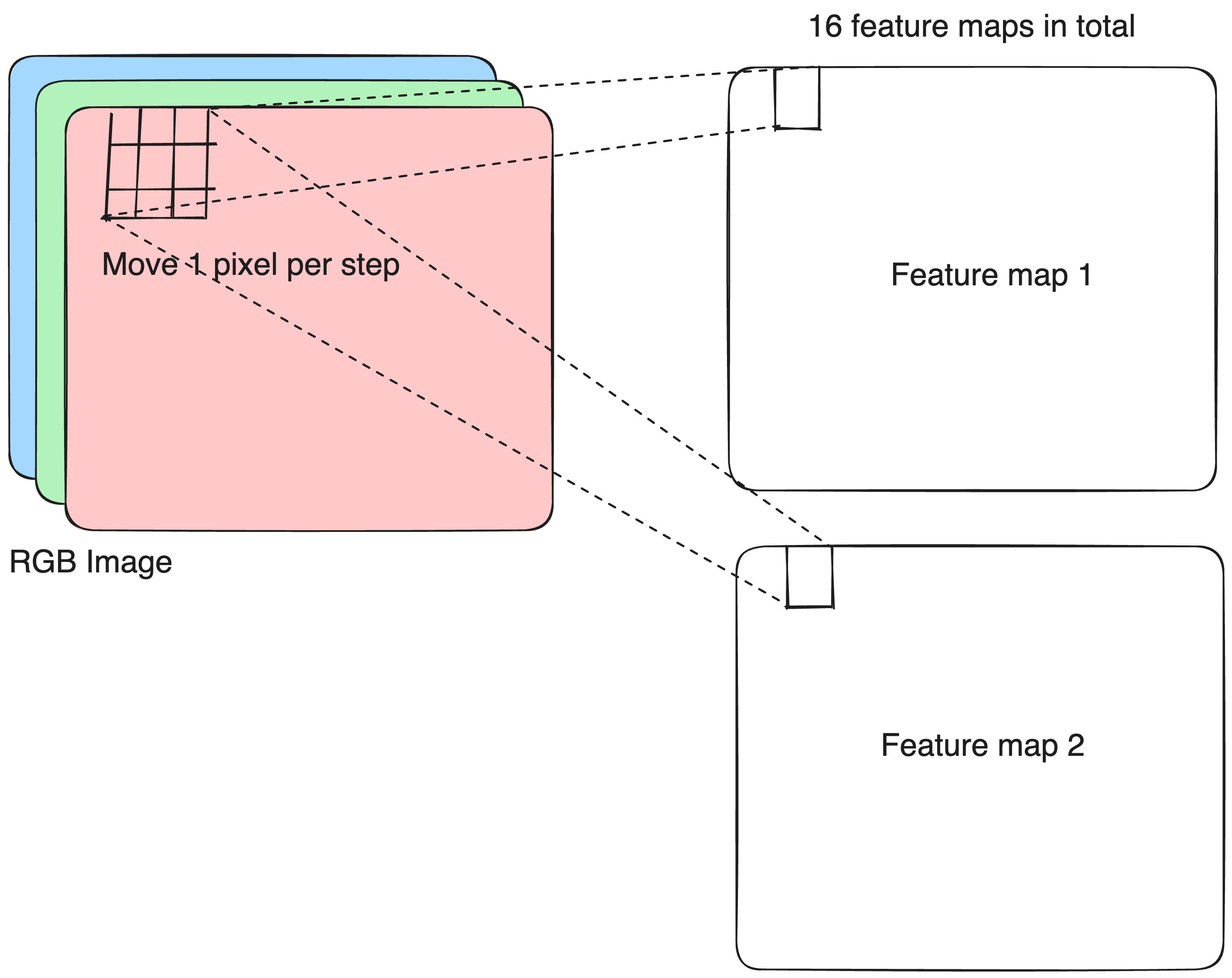
Conv2D layer
stridescontrols how far the kernel moves across the input in each step.
Conv2D layer
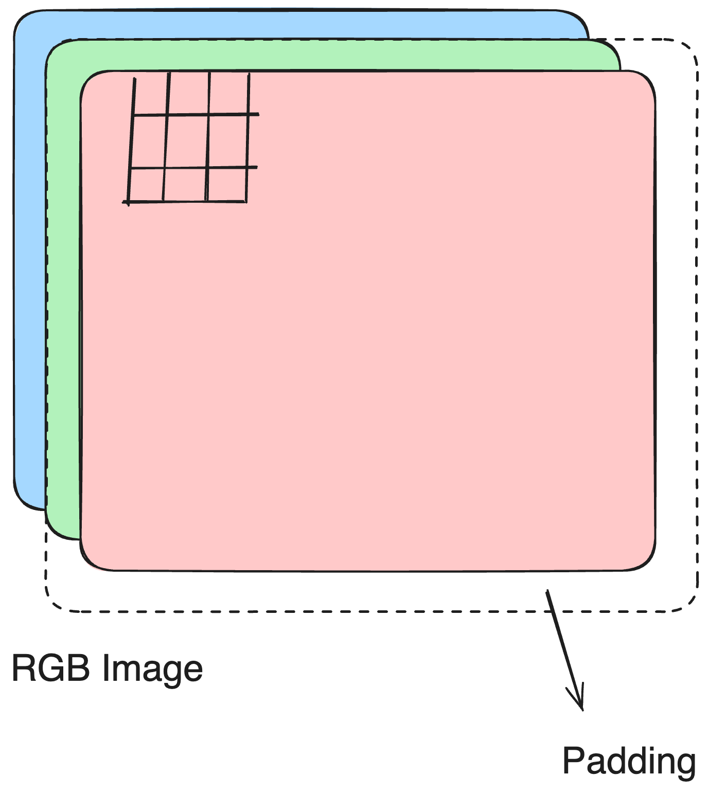
paddingdetermines how boundary pixels are handled.
padding = "same"keeps the output size equal to the input size.padding = "valid"means no padding is added, so the output is smaller.
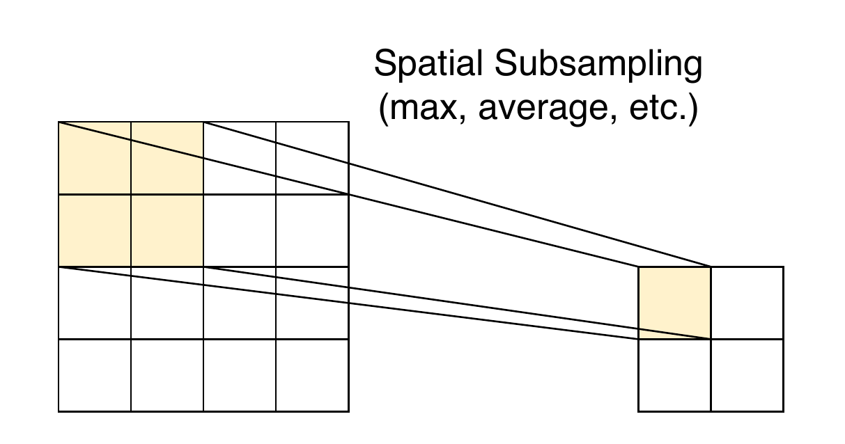
Spatial subsampling
Exact feature location is less important than relative position.
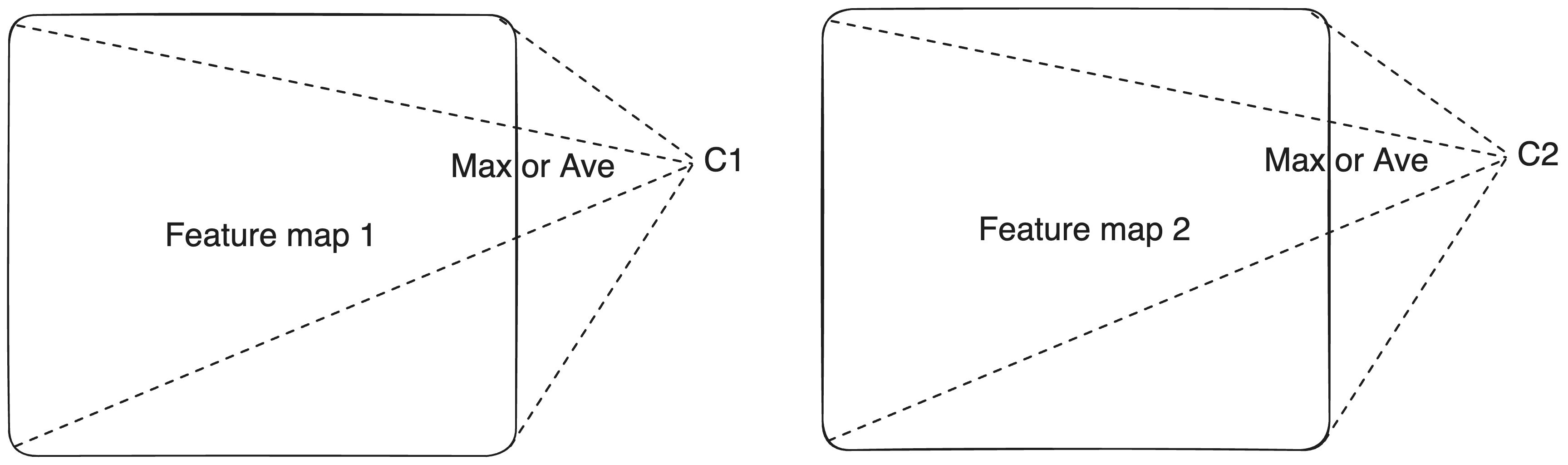
From feature maps to feature vectors
- This value can indicate whether a visual feature is present and how strongly it appears.
- It is position-invariant, meaning we don’t care where the feature occurs in the feature map.
- It also helps filter out noise and focus on the most important information.
Random crop
Random crop snips out a small window from the image at a random location to teach the model not to rely on exact spatial placement.
Before

keras$layers$RandomCrop

Random translation
Random translation shifts the image horizontally or vertically by a small random amount so the model doesn’t get hung up on exact positioning.
Before
keras$layers$RandomTranslation
![]()
Random shear
Random shear slants the image sideways by a random angle to help the model handle skewed or tilted shapes.
Before
keras$layers$RandomShear

Random rotation
Random rotation spins the image by a random angle so the model learns to recognize objects regardless of their orientation.
Before
keras$layers$RandomRotation

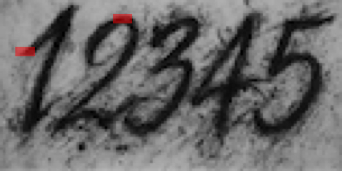
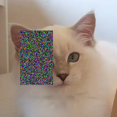
Random erasing
Random erasing randomly selects a rectangle region in an image and replaces its pixels with random values or a constant, simulating occlusion to improve model robustness.
Before
keras$layers$RandomErasing
Random color jitter
Random color jitter randomly changes an image’s brightness, contrast, saturation, and hue to simulate lighting variations and improve model generalization.
Before
keras$layers$RandomColorJitter

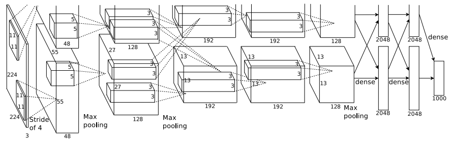
AlexNet (2012)
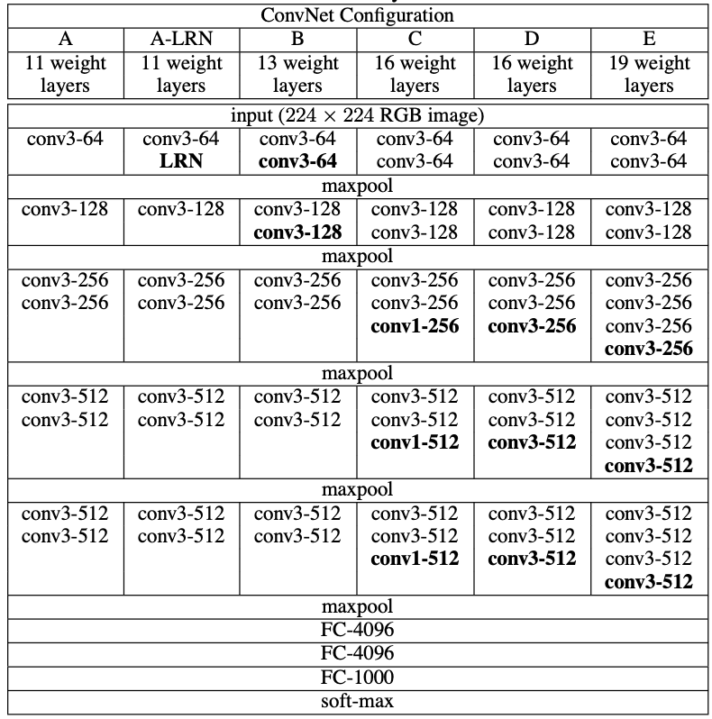
VGG (2014)
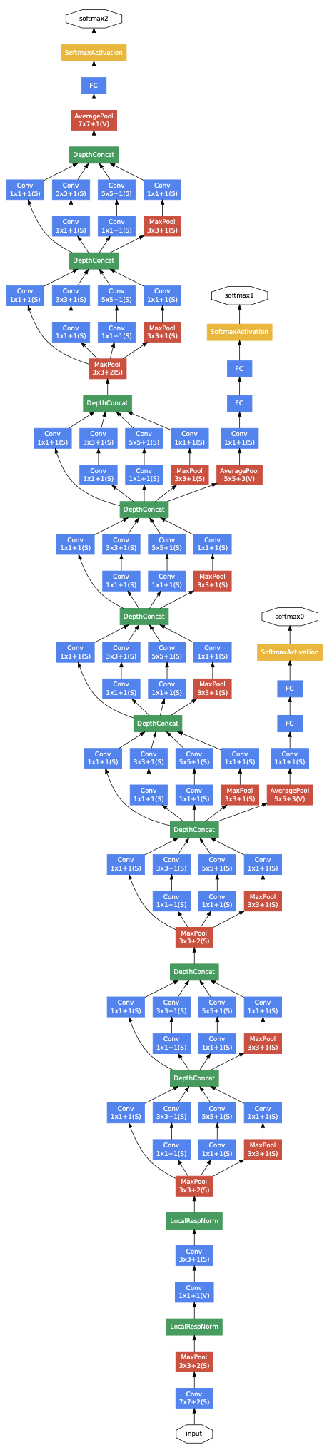
Inception (2014)
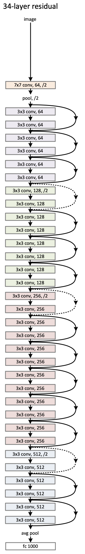
ResNet (2015)
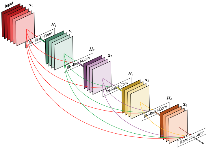
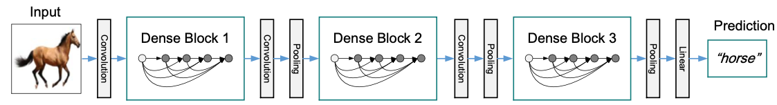
DenseNet (2016)
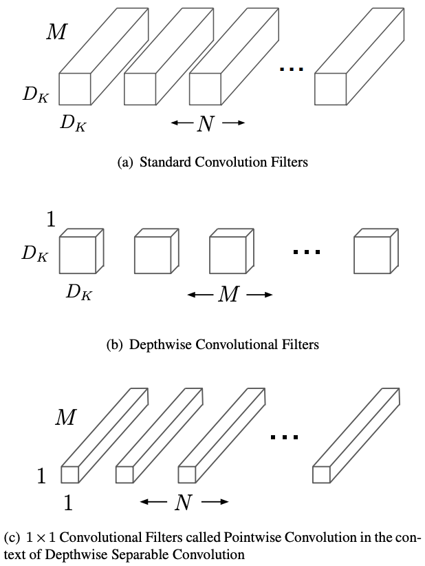
MobileNet (2017)
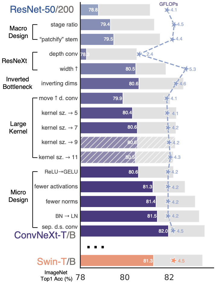
ConvNeXt (2022)
Exercises 2.2.2
Apply transfer learning with a pretrained ConvNeXtTiny backbone. On top of the backbone, add a domain adapter consisting of two convolutional layers with 32 filters, each followed by a batch normalization layer, and a final convolutional layer with 3 filters. After the ConvNeXtTiny feature extractor, apply global average pooling and connect it directly to the output layer.