Deep Learning and Computer Vision in R: A Practical Introduction (2.2)
BIBC2025 workshop - Image classification: Convolutional neural networks
Patrick Li
RSFAS, ANU
Content summary
- Overview of computer vision (CV)
reticulatebasics- > Image classification
- Hyperparameter tuning
- CV model interpretation
- Object detection
- Image segmentation
Convolutional neural networks
Why fully-connected NN struggle?
- High dimensionality: large input sizes lead to an explosion of parameters.
Model: "functional"
┏━━━━━━━━━━━━━━━━━━━━━━━━━━━━━━━━━┳━━━━━━━━━━━━━━━━━━━━━━━━┳━━━━━━━━━━━━━━━┓
┃ Layer (type)                    ┃ Output Shape           ┃       Param # ┃
┡━━━━━━━━━━━━━━━━━━━━━━━━━━━━━━━━━╇━━━━━━━━━━━━━━━━━━━━━━━━╇━━━━━━━━━━━━━━━┩
│ input_layer (InputLayer)        │ (None, 64, 64, 3)      │             0 │
├─────────────────────────────────┼────────────────────────┼───────────────┤
│ flatten (Flatten)               │ (None, 12288)          │             0 │
├─────────────────────────────────┼────────────────────────┼───────────────┤
│ dense (Dense)                   │ (None, 256)            │     3,145,984 │
├─────────────────────────────────┼────────────────────────┼───────────────┤
│ dense_1 (Dense)                 │ (None, 2)              │           514 │
└─────────────────────────────────┴────────────────────────┴───────────────┘
 Total params: 3,146,498 (12.00 MB)
 Trainable params: 3,146,498 (12.00 MB)
 Non-trainable params: 0 (0.00 B)
Why fully-connected NN struggle?
- No translation invariance: the same object in a different place looks completely different.
array([[0.4848306 , 0.51516944]], dtype=float32)array([[0.7504414 , 0.24955861]], dtype=float32)
Why fully-connected NN struggle?
- Ignored input topology: the spatial structure of images and local correlations are not inherently utilized.
Convolutional neural networks
A convolutional neural network typically consists of:
- Convolutional layers
- Subsampling (or pooling) layers
- Fully connected layers

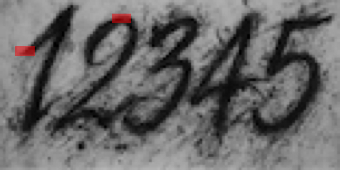
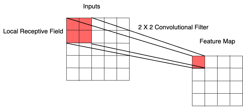
Local receptive fields
Convolutional layers connect each unit to a small local region of the previous layer.
Local receptive fields extract basic features (e.g. edges, corners), which are combined in deeper layers to detect higher order patterns.
Feature maps
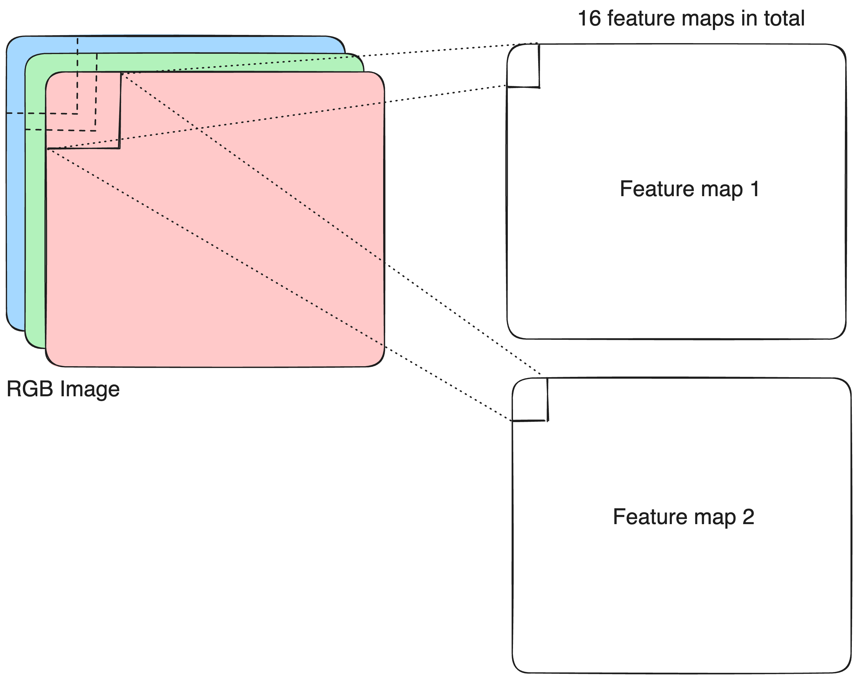
A convolutional layer typically produces multiple feature maps to capture different visual patterns.
Different filters extract different types of features from the same image:
- Image \rightarrow Convolutional layer 1, filter 1 \rightarrow edges
- Image \rightarrow Convolutional layer 1, filter 2 \rightarrow corners
- …
Deeper layers combine these elementary features to detect more complex patterns:
- Edges + corners + other features \rightarrow Convolutional layer 2, filter 1 \rightarrow eye
- Edges + corners + other features \rightarrow Convolutional layer 2, filter 2 \rightarrow mouth
- …
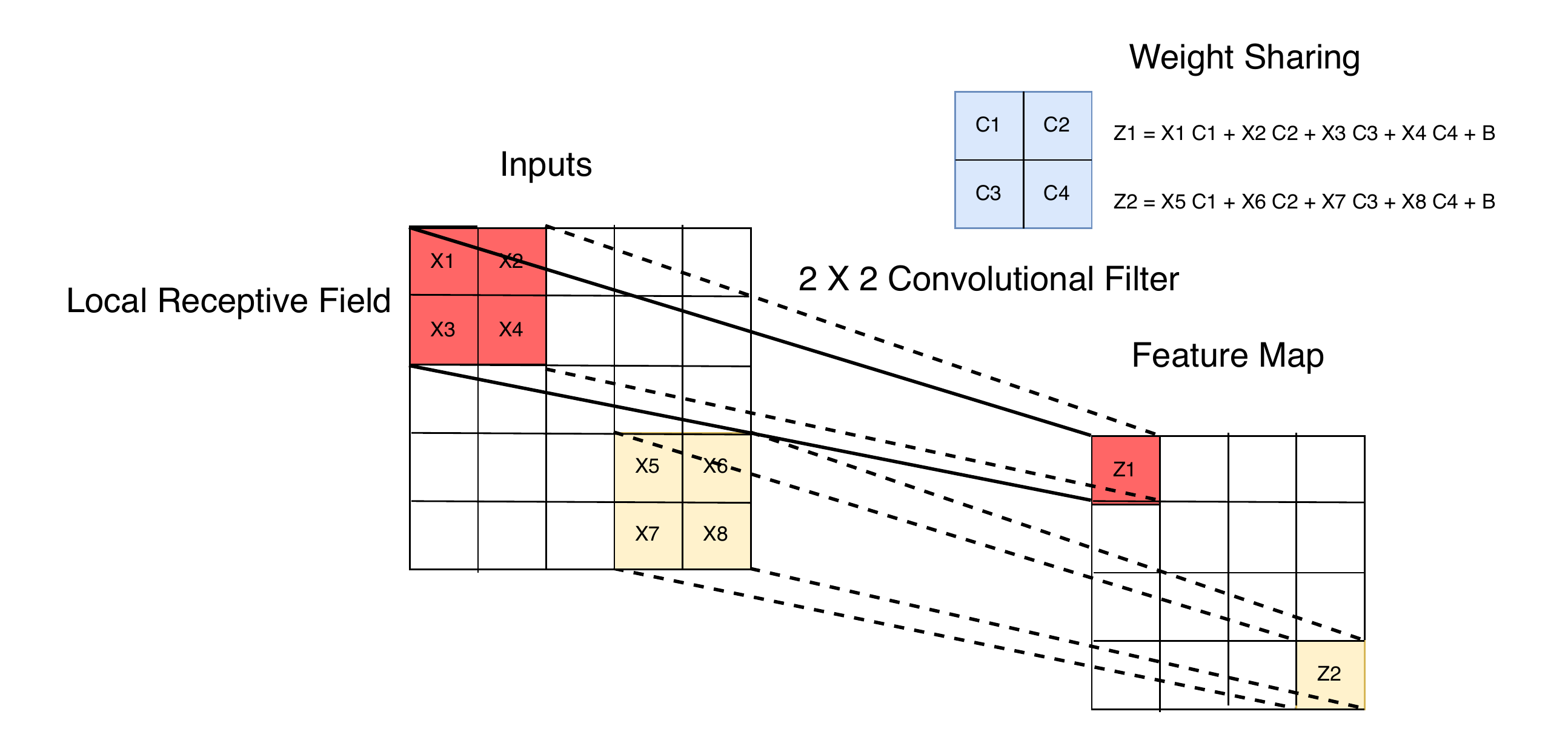
Weight sharing
Weight sharing
\text{Weight sharing} = \text{shift invariance} + \text{less parameters} + \text{smaller generalisation gap}
- Local feature detectors can be applied across the image using identical weights.
- Shifted inputs produce shifted feature maps, making CNNs robust to shifts and distortions.
- Weight sharing reduces model capacity, helping to reduce the train-test error gap.
Conv2D layer
filtersspecifies the number of convolutional filters (feature maps).
Conv2D layer
kernel_sizedefines the height and width of each convolutional filter.
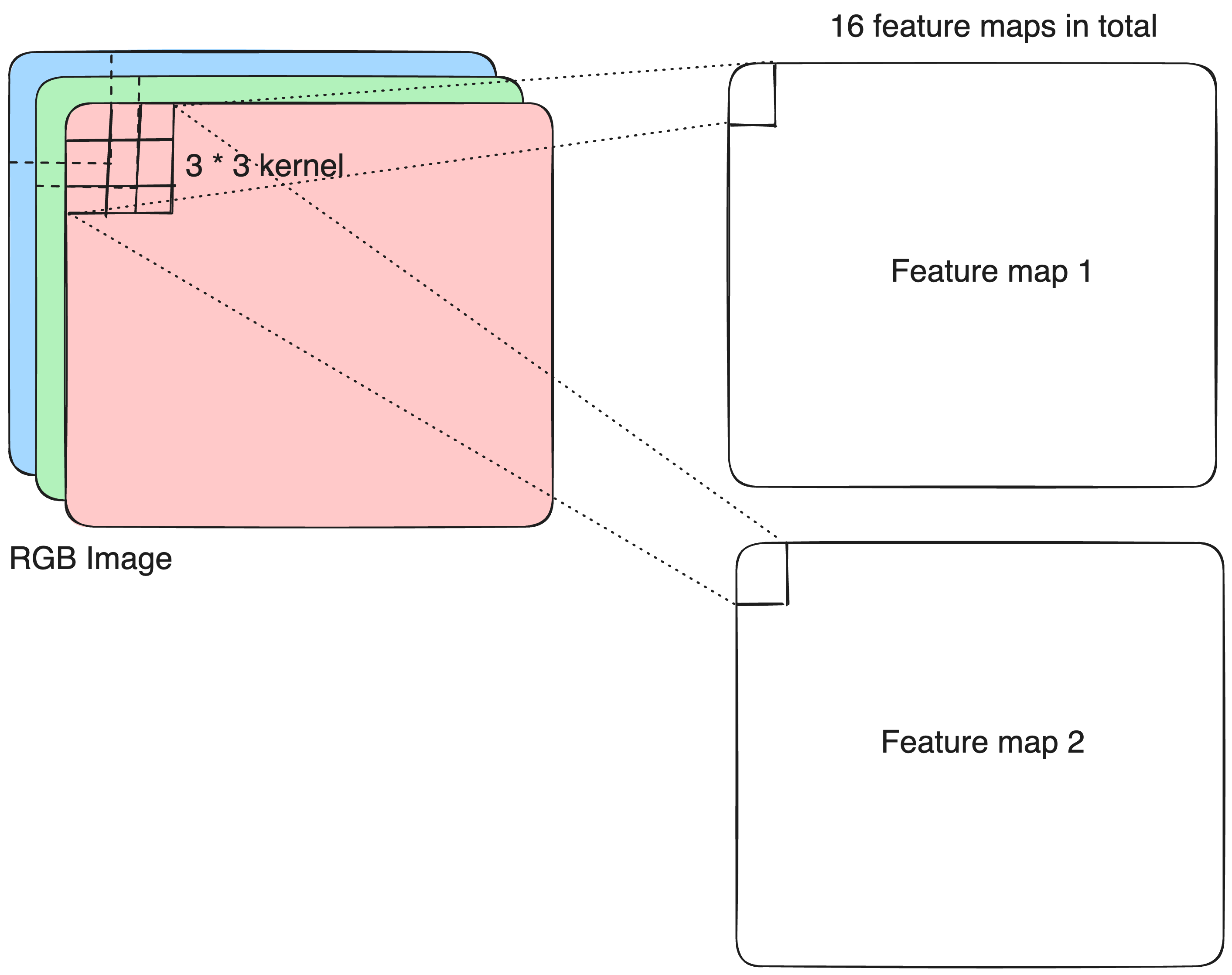
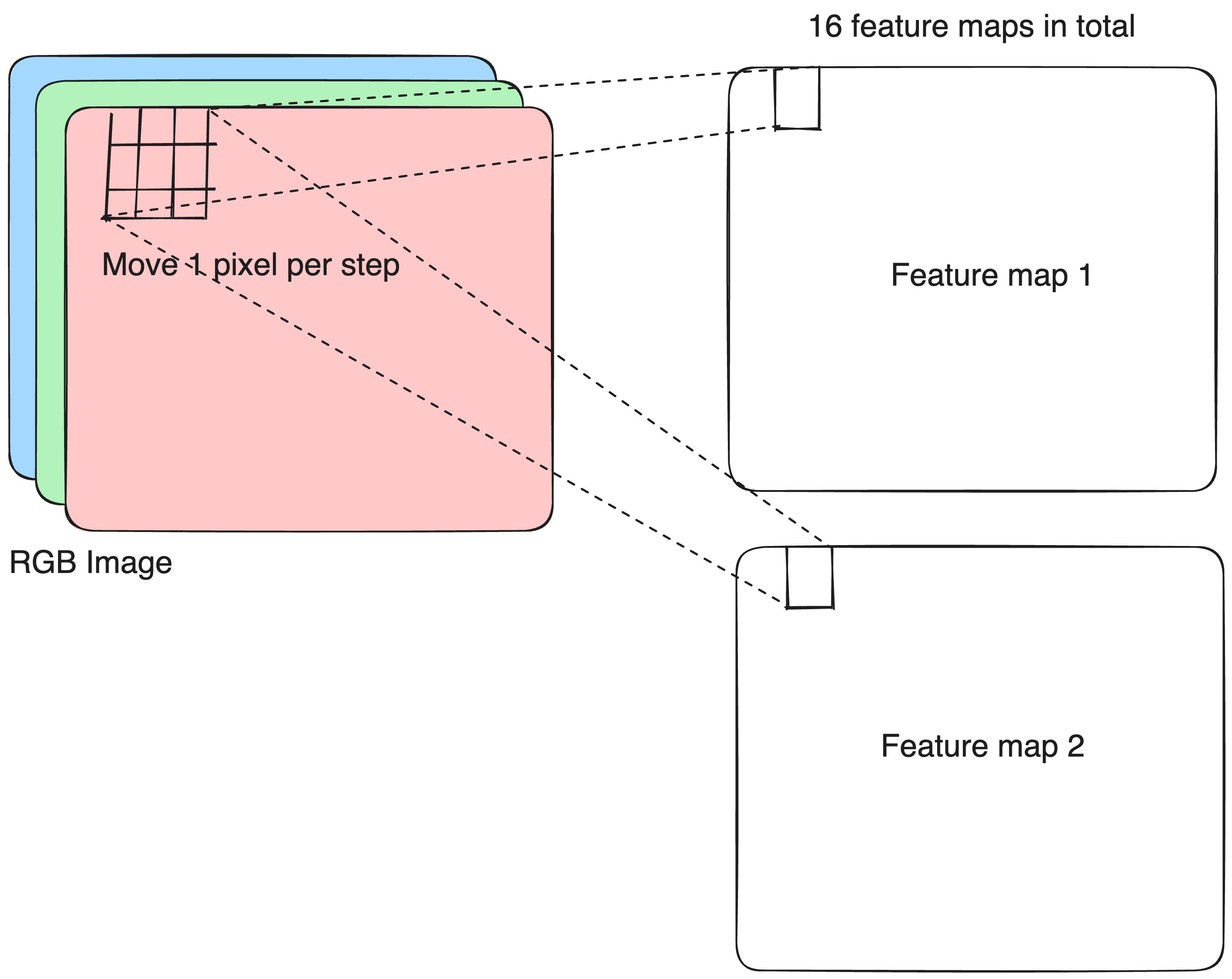
Conv2D layer
stridescontrols how far the kernel moves across the input in each step.
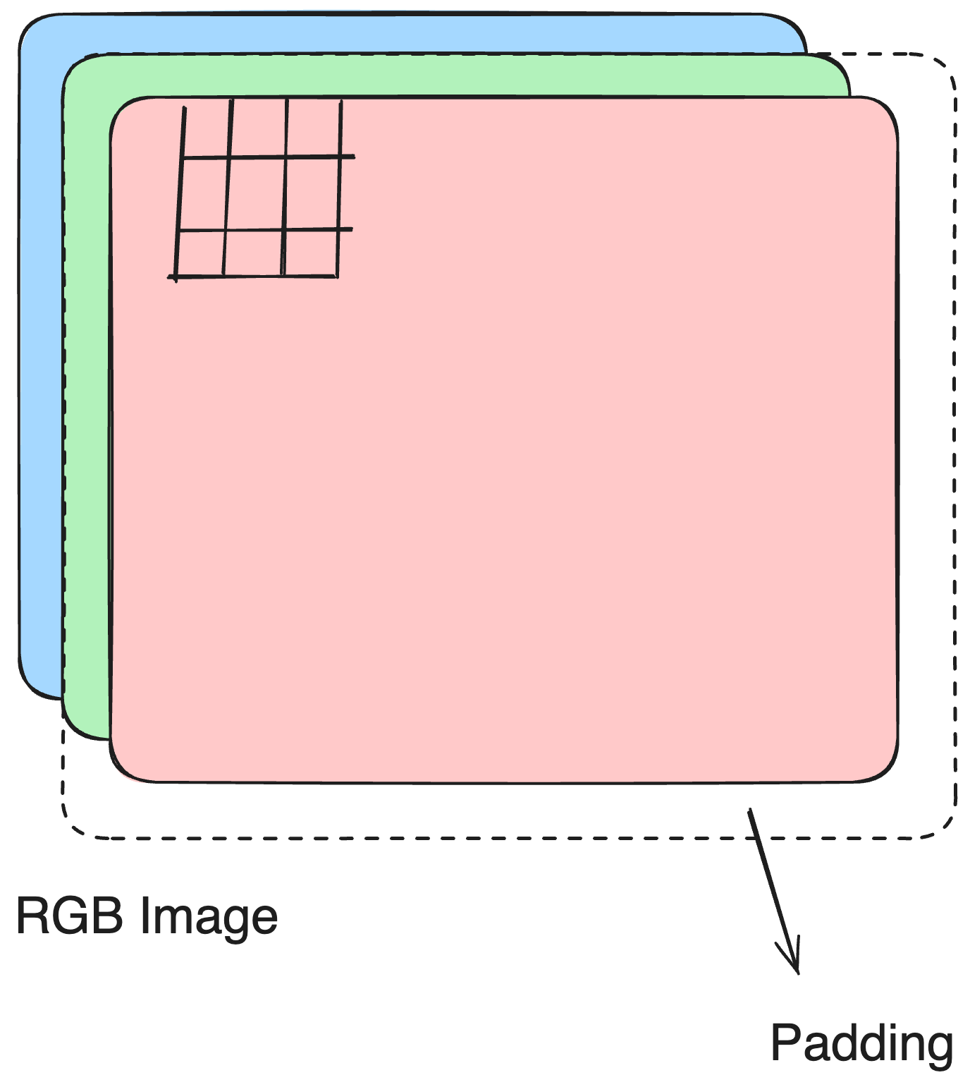
Conv2D layer
paddingdetermines how boundary pixels are handled.
padding = "same"keeps the output size equal to the input size.padding = "valid"means no padding is added, so the output is smaller.
Spatial subsampling
Pooling reduces resolution and sensitivity to small shifts and distortions by summarising information over local neighbourhoods.
Exact feature location is less important than relative position.
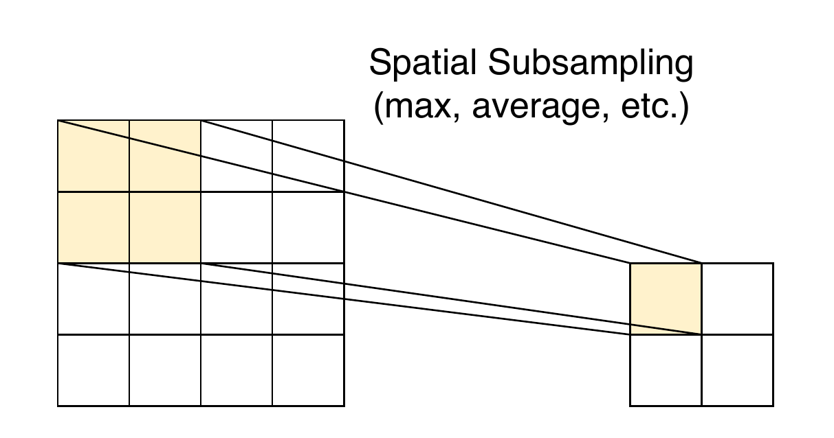
MaxPool2D & AveragePooling2D
pool_size controls the pooling window size and how it moves over the input.
Convolutional feature extractor
A typical convolutional feature extractor consists of several convolutional blocks (Conv2D + MaxPool2D). The end product is a (B, H, W, C) tensor.
conv_block <- \(x) {
  keras$layers$Conv2D(32L, tuple(3L, 3L), padding = "same")(x) |>
  keras$layers$ReLU()() |>
  keras$layers$MaxPool2D(tuple(2L, 2L))()
}

input <- keras$layers$Input(tuple(32L, 32L, 3L))

conv_block(input) |>
  conv_block() |>
  conv_block()
<KerasTensor shape=(None, 4, 4, 32), dtype=float32, sparse=False, ragged=False, name=keras_tensor_13>From feature maps to feature vectors
Global pooling extracts a single value from each channel to represent the entire feature map.
- This value can indicate whether a visual feature is present and how strongly it appears.
- It is position-invariant, meaning we don’t care where the feature occurs in the feature map.
- It also helps filter out noise and focus on the most important information.

Global pooling layers
GlobalMaxPool2D/GlobalAveragePooling2D: (B, H, W, C) \overset{\max/\text{ave}}{\longrightarrow} (B, C)
The output has now returned to our familiar matrix shape (2D tensor), so we could use the C features as predictors for classification.
Classifier head
Add a fully-connected NN as the classifier head on top of the feature extractor.
A simple CNN: complete workflow
conv_block <- \(x) {
  keras$layers$Conv2D(32L, tuple(3L, 3L), padding = "same")(x) |>
  keras$layers$ReLU()() |>
  keras$layers$MaxPool2D(tuple(2L, 2L))()
}

input <- keras$layers$Input(tuple(32L, 32L, 3L))

output <- conv_block(input) |>
  conv_block() |>
  conv_block() |>
  keras$layers$GlobalAveragePooling2D()() |>
  keras$layers$Dense(256L, activation = "relu")() |>
  keras$layers$Dense(1L, activation = "sigmoid")()

model <- keras$Model(input, output)
model$summary()
Model: "functional_1"
┏━━━━━━━━━━━━━━━━━━━━━━━━━━━━━━━━━┳━━━━━━━━━━━━━━━━━━━━━━━━┳━━━━━━━━━━━━━━━┓
┃ Layer (type) ┃ Output Shape ┃ Param # ┃
┡━━━━━━━━━━━━━━━━━━━━━━━━━━━━━━━━━╇━━━━━━━━━━━━━━━━━━━━━━━━╇━━━━━━━━━━━━━━━┩
│ input_layer_2 (InputLayer) │ (None, 32, 32, 3) │ 0 │
├─────────────────────────────────┼────────────────────────┼───────────────┤
│ conv2d_11 (Conv2D) │ (None, 32, 32, 32) │ 896 │
├─────────────────────────────────┼────────────────────────┼───────────────┤
│ re_lu_11 (ReLU) │ (None, 32, 32, 32) │ 0 │
├─────────────────────────────────┼────────────────────────┼───────────────┤
│ max_pooling2d_11 (MaxPooling2D) │ (None, 16, 16, 32) │ 0 │
├─────────────────────────────────┼────────────────────────┼───────────────┤
│ conv2d_10 (Conv2D) │ (None, 16, 16, 32) │ 9,248 │
├─────────────────────────────────┼────────────────────────┼───────────────┤
│ re_lu_10 (ReLU) │ (None, 16, 16, 32) │ 0 │
├─────────────────────────────────┼────────────────────────┼───────────────┤
│ max_pooling2d_10 (MaxPooling2D) │ (None, 8, 8, 32) │ 0 │
├─────────────────────────────────┼────────────────────────┼───────────────┤
│ conv2d_9 (Conv2D) │ (None, 8, 8, 32) │ 9,248 │
├─────────────────────────────────┼────────────────────────┼───────────────┤
│ re_lu_9 (ReLU) │ (None, 8, 8, 32) │ 0 │
├─────────────────────────────────┼────────────────────────┼───────────────┤
│ max_pooling2d_9 (MaxPooling2D) │ (None, 4, 4, 32) │ 0 │
├─────────────────────────────────┼────────────────────────┼───────────────┤
│ global_average_pooling2d_2 │ (None, 32) │ 0 │
│ (GlobalAveragePooling2D) │ │ │
├─────────────────────────────────┼────────────────────────┼───────────────┤
│ dense_5 (Dense) │ (None, 256) │ 8,448 │
├─────────────────────────────────┼────────────────────────┼───────────────┤
│ dense_4 (Dense) │ (None, 1) │ 257 │
└─────────────────────────────────┴────────────────────────┴───────────────┘
Total params: 28,097 (109.75 KB)
Trainable params: 28,097 (109.75 KB)
Non-trainable params: 0 (0.00 B)Exercises 2.2.1
- Train a CNN with a single convolutional block and a dense layer of 32 units.
- Extend the CNN to two convolutional blocks, and increase the units in dense layer to 256.
- Update the convolutional block function so that it can take two arguments:
- the number of convolutional layers, and
- the number of filters for those layers.
- a block with two convolutional layers, each using 32 filters
- a block with two convolutional layers, each using 64 filters
- a block with two convolutional layers, each using 128 filters Additionally, include a batchnormalization layer after every convolutional layer. After each pooling layer, except for the global pooling layer, add a dropout layer with a rate of 0.3.
- Compare the CNN’s performance with standard neural networks and other machine learning methods.
Image augmentation
Image augmentation expands your dataset by creating realistic variations, helping models become more robust and generalizable.
- Boost data diversity so models generalize better.
- Reduce overfitting, especially with smaller datasets.
- Mimic real-world variation such as rotation, lighting, scale, or noise.
You can define augmentations manually or learn them automatically, and apply them either once before training or dynamically during training.
Random crop
Random crop snips out a small window from the image at a random location to teach the model not to rely on exact spatial placement.
Before

keras$layers$RandomCrop

Random translation
Random translation shifts the image horizontally or vertically by a small random amount so the model doesn’t get hung up on exact positioning.
Before

keras$layers$RandomTranslation

Random shear
Random shear slants the image sideways by a random angle to help the model handle skewed or tilted shapes.
Before

keras$layers$RandomShear

Random rotation
Random rotation spins the image by a random angle so the model learns to recognize objects regardless of their orientation.
Before

keras$layers$RandomRotation

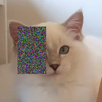
Random erasing
Random erasing randomly selects a rectangle region in an image and replaces its pixels with random values or a constant, simulating occlusion to improve model robustness.
Before

keras$layers$RandomErasing
Random color jitter
Random color jitter randomly changes an image’s brightness, contrast, saturation, and hue to simulate lighting variations and improve model generalization.
Before

keras$layers$RandomColorJitter

Landmark CNN architectures
LeNet-5 (1998)
%%{init: {'themeVariables': { 'fontSize': '43px'}}}%%
graph LR
    Input["Input<br/>32×32×1<br/>Grayscale"] --> C1["Conv2D<br/>6 filters<br/> 5×5<br/>Output: <br/>28×28×6"]
    C1 --> S2["AvePooling2D<br/> 2×2<br/>Output: <br/>14×14×6"]
    S2 --> C3["Conv2D<br/>16 filters<br/> 5×5<br/>Output: <br/>10×10×16"]
    C3 --> S4["AvePooling2D<br/> 2×2<br/>Output: <br/>5×5×16"]
    S4 --> C5["Conv2D<br/>120 filters<br/> 5×5<br/>Output: <br/>1×1×120<br/>"]
    C5 --> F6["Dense<br/>84 units<br/>tanh"]
    F6 --> Output["Output Layer<br/>10 units<br/>Classes 0-9"]

    classDef convLayer fill:#e1f5fe,stroke:#01579b,stroke-width:2px
    classDef poolLayer fill:#f3e5f5,stroke:#4a148c,stroke-width:2px
    classDef fcLayer fill:#e8f5e8,stroke:#1b5e20,stroke-width:2px
    classDef inputOutput fill:#fff3e0,stroke:#e65100,stroke-width:2px

    class Input,Output inputOutput
    class C1,C3,C5 convLayer
    class S2,S4 poolLayer
    class F6 fcLayer
- More feature maps at lower resolution to build invariance.
- Standardised inputs for faster, more stable training.
- No padding, so feature maps shrink after each conv.
tanhactivations throughout.- Prototype-based final layer using Euclidean distance, yielding low out-of-distribution activations.
- Trained with stochastic Levenberg–Marquardt (diagonal Hessian approximation).
- Training performed on a single R10000 CPU.
AlexNet (2012)

- 61M parameters; Deeper and wider than earlier CNNs; first big proof that scale wins.
- ReLU activations for significantly faster training.
- Local Response Normalization (lateral inhibition) promotes channel-wise competition.
- Dropout in dense layers to reduce overfitting.
- PCA-based color augmentation for data enrichment.
- Trained with stochastic gradient descent (SGD) + momentum.
- Two GTX580 used to train the model because one GPU couldn’t fit everything.
VGG (2014)
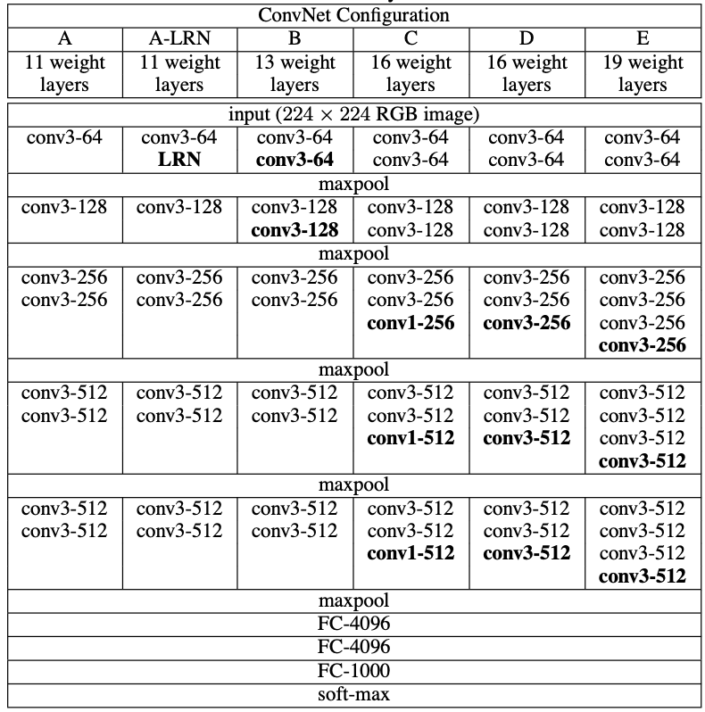
- Much deeper (16–19 layers) \rightarrow captures more complex features.
- Uniform 3×3 convolutions \rightarrow simulates larger receptive fields efficiently.
- More parameters (138-144M).
- Simpler design (no LRN) \rightarrow easier to scale and reproduce.
- Input preprocessing: resized to 224×224, mean-subtracted, random crops and horizontal flips for augmentation.
- Inference trick: multi-crop / multi-scale averaging to improve accuracy.
Inception (2014)

- Inception modules combine 1×1, 3×3, 5×5 convs + pooling in parallel \rightarrow captures multi-scale features efficiently.
- 1×1 convolutions as dimension reduction module \rightarrow massive parameter and FLOP reduction.
- Very deep (22 layers) but only ~6.8M parameters.
- Spatial dimension preserved via carefully arranged pooling and reduction.
- Auxiliary classifiers in the middle of the network \rightarrow help gradient flow and regularization.
- LRN used, similar to AlexNet.
ResNet (2015)

- Residual (skip) connections: allow layers to learn residual functions \mathcal{F}(X) + X, enabling training of extremely deep networks (18-152 layers, 11-60M parameters) without degradation.
- Bottleneck design (for 50+ layers): 1×1 \rightarrow 3×3 \rightarrow 1×1 convolutions in each residual block.
- Batch Normalization after every convolution for stable and faster training.
- Global average pooling before the final fully connected layer \rightarrow reduces parameters compared with VGG.
DenseNet (2016)
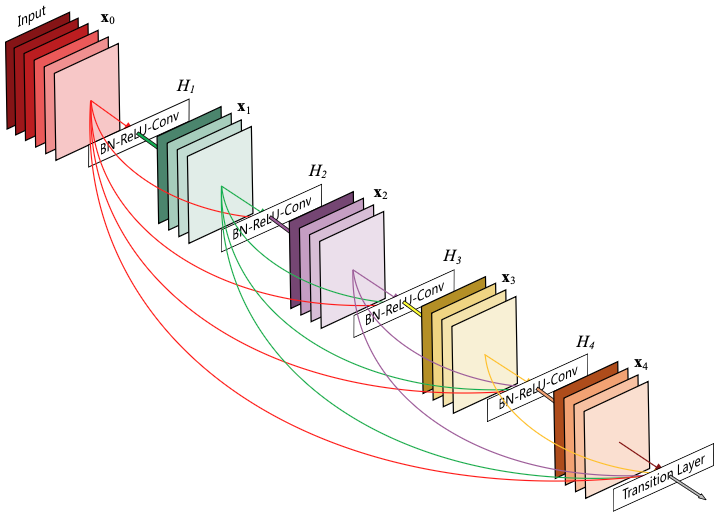

- Dense connectivity: each layer receives all previous feature maps as input and passes its output forward, massively improving gradient flow and feature reuse.
- Growth rate: controls how many new feature maps each layer contributes, letting DenseNet stay surprisingly compact (121-264 layers, 8–33M parameters).
- Bottleneck + compression: 1×1 bottleneck layers and channel compression in transition layers keep computation manageable.
MobileNet (2017)
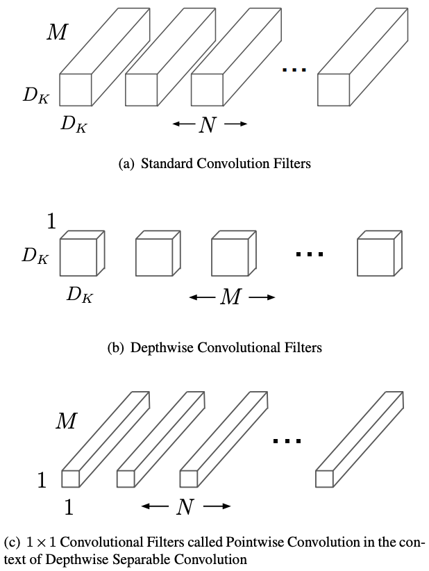
- Depthwise separable convolutions: splits standard convolution into depthwise (per-channel) and pointwise (1×1) operations, reducing parameters by 8-9× with minimal accuracy loss.
- K^2C_{\text{in}}C_{\text{out}} \rightarrow K^2C_{\text{in}} + C_{\text{in}}C_{\text{out}}
- Designed for mobile: optimized for edge devices with limited compute, enabling real-time inference on smartphones (3-5M parameters, <300M FLOPs).
ConvNeXt (2022)
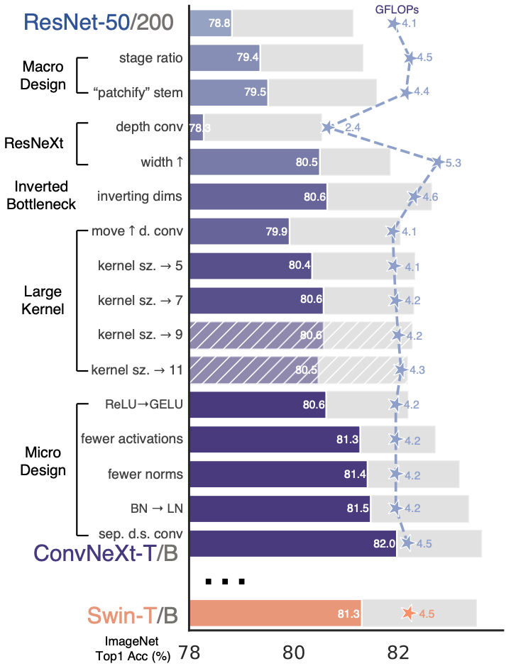
Starting from ResNet-50 (76.1%), ending with vision transformer performance!
- Training techniques (→78.8%): AdamW, Mixup/Cutmix, stochastic depth, label smoothing
- Macro design (→79.4%): Stage compute ratio (3,3,9,3) like Swin Transformer
- Depthwise convolutions (→80.5%)
- Large kernels (→81.3%): 7×7 convs for larger receptive field (approaching ViT’s global attention)
- Micro designs (→82.0%): GELU, fewer activations/normalizations, LayerNorm instead of BatchNorm, layer scaling
Pre-trained model in keras
Getting a common pre-trained CNN on ImageNet is very simple with keras$applications. It just pulls the checkpoint for you and caches it locally, so you only download it once.
Model: "vgg16"
┏━━━━━━━━━━━━━━━━━━━━━━━━━━━━━━━━━┳━━━━━━━━━━━━━━━━━━━━━━━━┳━━━━━━━━━━━━━━━┓
┃ Layer (type)                    ┃ Output Shape           ┃       Param # ┃
┡━━━━━━━━━━━━━━━━━━━━━━━━━━━━━━━━━╇━━━━━━━━━━━━━━━━━━━━━━━━╇━━━━━━━━━━━━━━━┩
│ input_layer_3 (InputLayer)      │ (None, 224, 224, 3)    │             0 │
├─────────────────────────────────┼────────────────────────┼───────────────┤
│ block1_conv1 (Conv2D)           │ (None, 224, 224, 64)   │         1,792 │
├─────────────────────────────────┼────────────────────────┼───────────────┤
│ block1_conv2 (Conv2D)           │ (None, 224, 224, 64)   │        36,928 │
├─────────────────────────────────┼────────────────────────┼───────────────┤
│ block1_pool (MaxPooling2D)      │ (None, 112, 112, 64)   │             0 │
├─────────────────────────────────┼────────────────────────┼───────────────┤
│ block2_conv1 (Conv2D)           │ (None, 112, 112, 128)  │        73,856 │
├─────────────────────────────────┼────────────────────────┼───────────────┤
│ block2_conv2 (Conv2D)           │ (None, 112, 112, 128)  │       147,584 │
├─────────────────────────────────┼────────────────────────┼───────────────┤
│ block2_pool (MaxPooling2D)      │ (None, 56, 56, 128)    │             0 │
├─────────────────────────────────┼────────────────────────┼───────────────┤
│ block3_conv1 (Conv2D)           │ (None, 56, 56, 256)    │       295,168 │
├─────────────────────────────────┼────────────────────────┼───────────────┤
│ block3_conv2 (Conv2D)           │ (None, 56, 56, 256)    │       590,080 │
├─────────────────────────────────┼────────────────────────┼───────────────┤
│ block3_conv3 (Conv2D)           │ (None, 56, 56, 256)    │       590,080 │
├─────────────────────────────────┼────────────────────────┼───────────────┤
│ block3_pool (MaxPooling2D)      │ (None, 28, 28, 256)    │             0 │
├─────────────────────────────────┼────────────────────────┼───────────────┤
│ block4_conv1 (Conv2D)           │ (None, 28, 28, 512)    │     1,180,160 │
├─────────────────────────────────┼────────────────────────┼───────────────┤
│ block4_conv2 (Conv2D)           │ (None, 28, 28, 512)    │     2,359,808 │
├─────────────────────────────────┼────────────────────────┼───────────────┤
│ block4_conv3 (Conv2D)           │ (None, 28, 28, 512)    │     2,359,808 │
├─────────────────────────────────┼────────────────────────┼───────────────┤
│ block4_pool (MaxPooling2D)      │ (None, 14, 14, 512)    │             0 │
├─────────────────────────────────┼────────────────────────┼───────────────┤
│ block5_conv1 (Conv2D)           │ (None, 14, 14, 512)    │     2,359,808 │
├─────────────────────────────────┼────────────────────────┼───────────────┤
│ block5_conv2 (Conv2D)           │ (None, 14, 14, 512)    │     2,359,808 │
├─────────────────────────────────┼────────────────────────┼───────────────┤
│ block5_conv3 (Conv2D)           │ (None, 14, 14, 512)    │     2,359,808 │
├─────────────────────────────────┼────────────────────────┼───────────────┤
│ block5_pool (MaxPooling2D)      │ (None, 7, 7, 512)      │             0 │
├─────────────────────────────────┼────────────────────────┼───────────────┤
│ flatten (Flatten)               │ (None, 25088)          │             0 │
├─────────────────────────────────┼────────────────────────┼───────────────┤
│ fc1 (Dense)                     │ (None, 4096)           │   102,764,544 │
├─────────────────────────────────┼────────────────────────┼───────────────┤
│ fc2 (Dense)                     │ (None, 4096)           │    16,781,312 │
├─────────────────────────────────┼────────────────────────┼───────────────┤
│ predictions (Dense)             │ (None, 1000)           │     4,097,000 │
└─────────────────────────────────┴────────────────────────┴───────────────┘
 Total params: 138,357,544 (527.79 MB)
 Trainable params: 138,357,544 (527.79 MB)
 Non-trainable params: 0 (0.00 B)
Transfer learning
Transfer Learning uses knowledge from a model trained on one task to improve learning and performance on a different but related task.
Why it works:
- Pre-trained models have already learned useful feature representations from large datasets.
- Early layers capture general features (edges, textures) that transfer well across tasks.
- Later layers can be fine-tuned for task-specific patterns, reducing training time and data needs.
Transfer learning: feature extraction
Feature extraction freezes convolutional blocks, and retrain only the final layers, enabling fast training and strong performance on small dataset.
Freeze the entire VGG16 network.
Transfer learning: fine-tuning
Fine-tuning retrains some of the later convolutional layers of a pre-trained network, allowing the model to adapt to a new task and often achieve higher accuracy.
Freeze the entire VGG16 network, except for the last convolutional block.
input <- keras$layers$Input(tuple(32L, 32L, 3L))
vgg16 <- keras$applications$VGG16(include_top = FALSE,
                                  input_tensor = input,
                                  pooling = "avg")
vgg16$trainable <- FALSE
py_for(layer ~ vgg16$layers[-5:-2], {
  layer$trainable <- TRUE
})
output <- keras$layers$Dense(1L, activation = "sigmoid")(vgg16(input))
keras$Model(input, output)
Exercises 2.2.2
Apply transfer learning with a pretrained ConvNeXtTiny backbone. On top of the backbone, add a domain adapter consisting of two convolutional layers with 32 filters, each followed by a batch normalization layer, and a final convolutional layer with 3 filters. After the ConvNeXtTiny feature extractor, apply global average pooling and connect it directly to the output layer.

Slides URL: https://ibsar-cv-workshop.patrickli.org/ | Canberra time