Deep Learning and Computer Vision in R: A Practical Introduction (2.1)

BIBC2025 workshop - Image classification: Introduction

Patrick Li

RSFAS, ANU

Content summary

• Overview of computer vision (CV)
• reticulate basics
• > Image classification
• Hyperparameter tuning
• CV model interpretation
• Object detection
• Image segmentation

Starting with image classification

Image classification is the task of assigning one or more category labels to an input image based on its visual content.

• Simplicity: It is the simplest and most fundamental vision task, helping models to extract and organise visual patterns like edges, shapes, and textures into meaningful object representations.

• Historical motivations: Researchers started with image classification because it isolates the core challenge of visual representation learning without the added complexity of where objects appear or how they are structured.

Pixels

Pixel is the smallest unit of an image, representing a single point of colour.

• Each pixel stores intensity information for one or more channels, depending on the colour scheme.

• The resolution of an image is given by the number of pixels along width \times height, e.g., 1920×1080.

A 32 \times 32 image

Colour schemes: greyscale

In greyscale image, each pixel stores one intensity value representing brightness.

• Typically represented as 0–255 (8-bit), where 0 = black, 255 = white.
• No colour information, only lightness/darkness.

A greyscale image

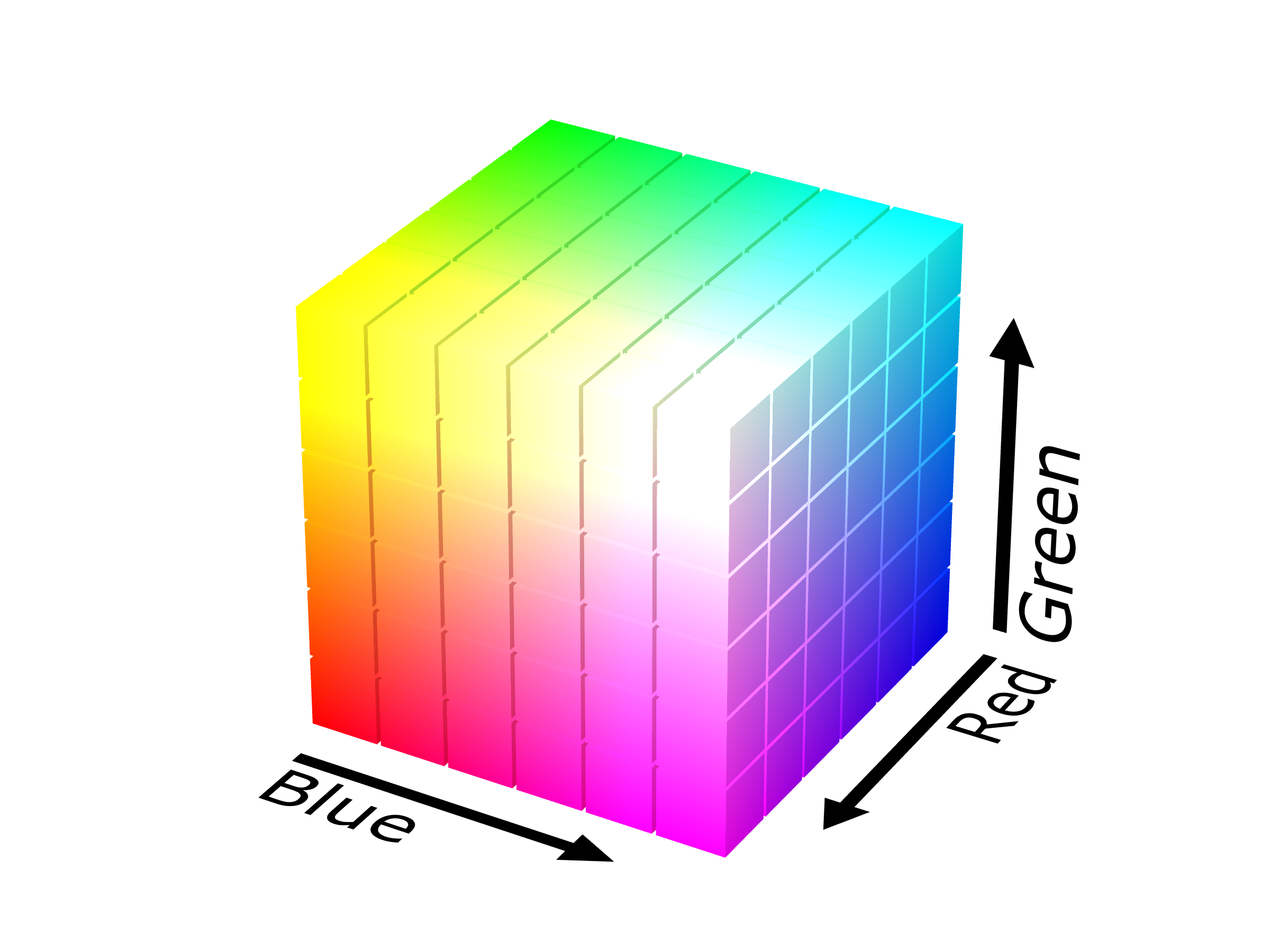
Colour schemes: RGB

In RGB image, each pixel has three channels: Red (R), Green (G) and Blue (B).

• Each channel is usually 8-bit (0 – 255), representing the intensity of that colour component.
• Variants:
  • RGBA: Adds an Alpha channel for transparency.
  • BGR: Some libraries (like OpenCV) use this channel order.

RGB cube

Colour schemes: others

• HSV / HSL: Occasionally used in image editing or visualisation tools, but rarely as a native storage format.
• YCbCr / YUV: Common in JPEG and video codecs (MPEG, H.264); separates brightness and colour for better compression.
• CMYK: Used in TIFF, EPS, and PDF formats for printing workflows.
• LAB (CIELAB): Supported in TIFF and PSD (Photoshop) for high-fidelity colour management.
• YCoCg: Used in some lossless video compression methods (e.g., H.264/AVC), a more efficient variant of YCbCr.
• Indexed colour / Palette-based (P): Stores a colour lookup table (palette) with pixel indices; common in GIF and PNG-8.

File types

File storage can differ from in-memory representation, because files often compress or encode the pixel data.

Extension	Typical Use	Notes
.jpg	Photographs	Compressed (lossy), reduces file size
.png	Graphics / web	Lossless, supports transparency (alpha channel)
.bmp	Windows bitmaps	Uncompressed, large file size
.tiff	High-quality images	Often used in printing or scientific imaging
.gif	Simple animations	256 colours only
.raw	Camera sensor data	Direct sensor output, unprocessed

In-memory representation

Once loaded into a program (Python, R, etc.), images are usually represented as multi-dimensional arrays/tensors in uint8 (0 - 255) or float32 (0 - 1).

• Greyscale image: 2D array [height, width]

torch$rand(100L, 100L)

• RGB image: 3D array [height, width, channels]

torch$rand(100L, 100L, 3L)

• Pay attention to the channel order
  • channels first [C, H, W]
  • channels last [H, W, C].

Image loading: classification

• Define the image dataset
• Loda images from dataset

ImageFolder expects a folder structure like this:

root/dog/xxx.png
root/dog/xxy.png
root/cat/123.png
root/cat/nsdf3.png

Once the images are loaded, we convert them to torch tensors stored in a torch Dataset.

tv <- import("torchvision", convert = FALSE)
dataset <- tv$datasets$ImageFolder(root = here::here("data/sample_images"),
                                   transform = tv$transforms$ToTensor())

DataLoader can sample images from a torch Dataset. We can create a wrapper around it to convert images to channel-last format and ensure they are on the desired device, such as a GPU.

device <- torch$accelerator$current_accelerator()
dataloader <- torch$utils$data$DataLoader(dataset, 
                                          batch_size = 10L, 
                                          shuffle = TRUE)

my_loader <- py_iterable_wrapper(dataloader, \(batch) {
  batch[0] <- batch[0]$permute(0L, 2L, 3L, 1L)
  batch[0] <- batch[0]$to(device = device, dtype = torch$float32)
  batch[1] <- batch[1]$to(device = device, dtype = torch$float32)
  return(tuple(batch[0], batch[1]))
})

py_for(c(x, y) ~ my_loader, {
  print(glue::glue("Images: {x$shape}, {x$dtype}, {x$device}"))
  print(glue::glue("Labels: {y$shape}, {y$dtype}, {y$device}"))
  break
})

Images: torch.Size([10, 2100, 2100, 3]), torch.float32, mps:0
Labels: torch.Size([10]), torch.float32, mps:0

Image loading: regression

For regression tasks, the image loading pipeline can be a bit more complicated, as it requires manually defining the dataset construction.

We won’t cover it in this workshop, but more details are available on https://docs.pytorch.org/tutorials/beginner/basics/data_tutorial.html#creating-a-custom-dataset-for-your-files.

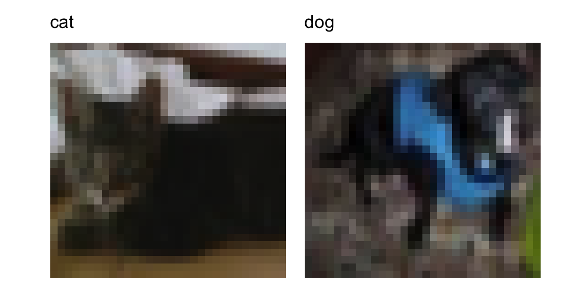
CIFAR datasets: Cat vs. Dog

The CIFAR datasets are widely used benchmarks for image recognition, containing labelled 32 \times 32 RGB images across multiple object categories.

We extract the cat and dog images from the dataset, using 5,000 for training and 2,000 for testing in each class.

Exercises 2.1.1:

1. Visualise the cat and dog images with map(), plot_rgb(), and wrap_plots().
2. Perform principal component analysis (PCA) on the training data.
3. Train logistic regression, linear discriminant analysis (LDA), quadratic discriminant analysis (QDA), and random forest models on the training set.
4. Evaluate model performance on the test set and compare results using ROC curves.

General machine learning methods

From the exercises:

• Flexible models are needed for vision tasks, as the problem is too complex for linear models to handle.
• Flexible models can easily overfit, so regularisation or parameter control is necessary to balance fit and generalisation.
• Baseline models such as QDA and random forest achieve 63 – 66% test accuracy.

Neural networks

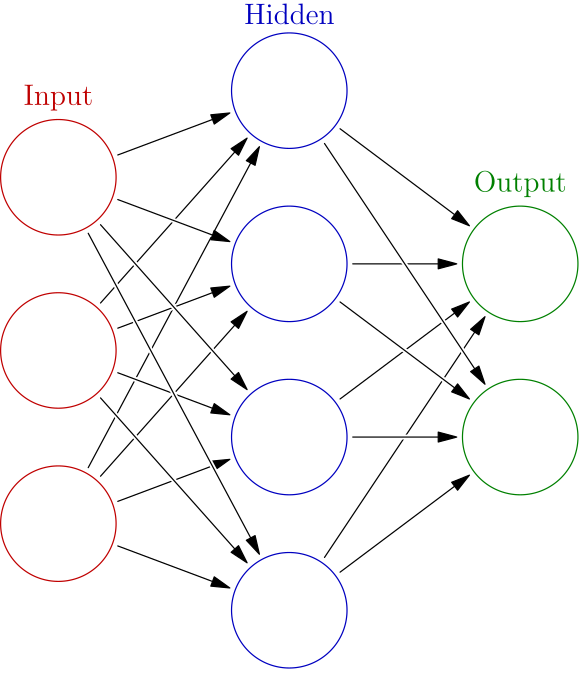
Neural networks

A neural network is a computational model composed of interconnected layers of nodes that learn to recognise patterns and relationships in data.

An artificial neural network

Neural networks

A general mathematical form of a neural network can be written as:

\mathbf{y} = f^{(L)}\Big(\mathbf{W}^{(L)} f_{\dots}\big(f^{(2)}(\mathbf{W}^{(2)} f^{(1)}(\mathbf{W}^{(1)} \mathbf{x} + \mathbf{b}^{(1)}) + \mathbf{b}^{(2)})\big) + \mathbf{b}^{(L)} \Big)

where:

• \mathbf{x} is the input vector,
• \mathbf{W}^{(\ell)} and \mathbf{b}^{(\ell)} are the weight matrix and bias vector at layer \ell,
• f^{(\ell)} is the activation function at layer \ell,
• L is the total number of layers,
• \mathbf{y} is the network output.

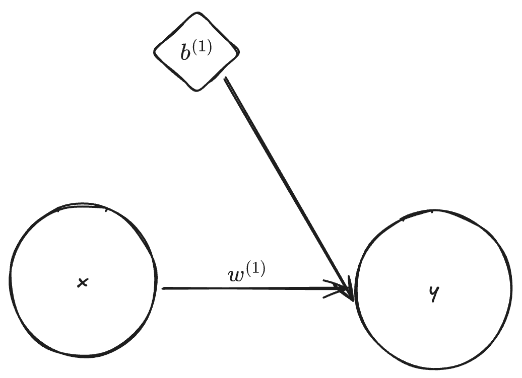
Simple linear regression

By setting the dimension of \mathbf{x}, \mathbf{y} and \mathbf{b}^{(1)} to one, L = 1 and f^{(1)}(z) = z, we obtain

y = w^{(1)} x + b^{(1)}.

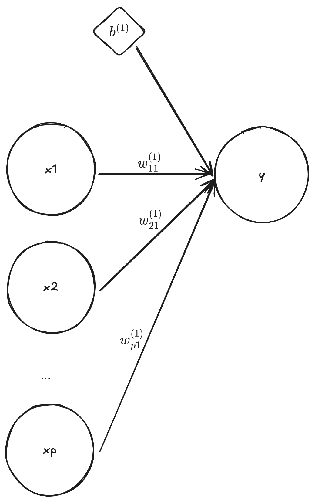
Multiple linear regression

By setting the dimension of \mathbf{x} to p, the dimension of \mathbf{y} and \mathbf{b}^{(1)} to one, L = 1 and f^{(1)}(z) = z, we obtain

y = \mathbf{w}^{(1)} \mathbf{x} + b^{(1)}.

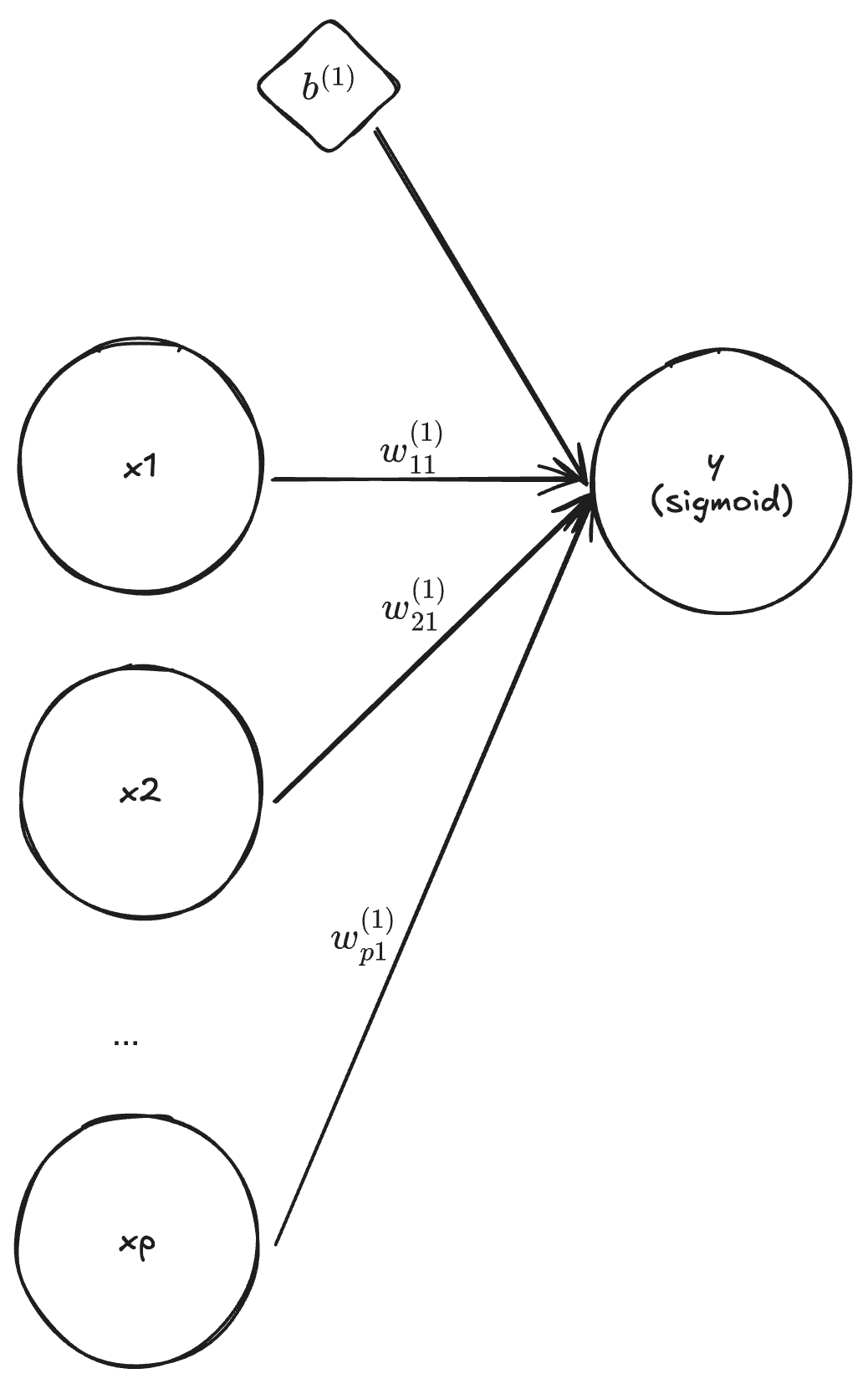
Logistic regression

By setting the dimension of \mathbf{x} to p, the dimension of \mathbf{y} and \mathbf{b}_1 to one, L = 1 and f^{(1)}(z) = \frac{e^z}{1 + e^z}, we obtain

y = f^{(1)}(\mathbf{W}^{(1)} \mathbf{x} + b^{(1)}) = \frac{e^{\mathbf{W}^{(1)} \mathbf{x} + b^{(1)}}}{1 + e^{\mathbf{W}^{(1)} \mathbf{x} + b^{(1)}}}.

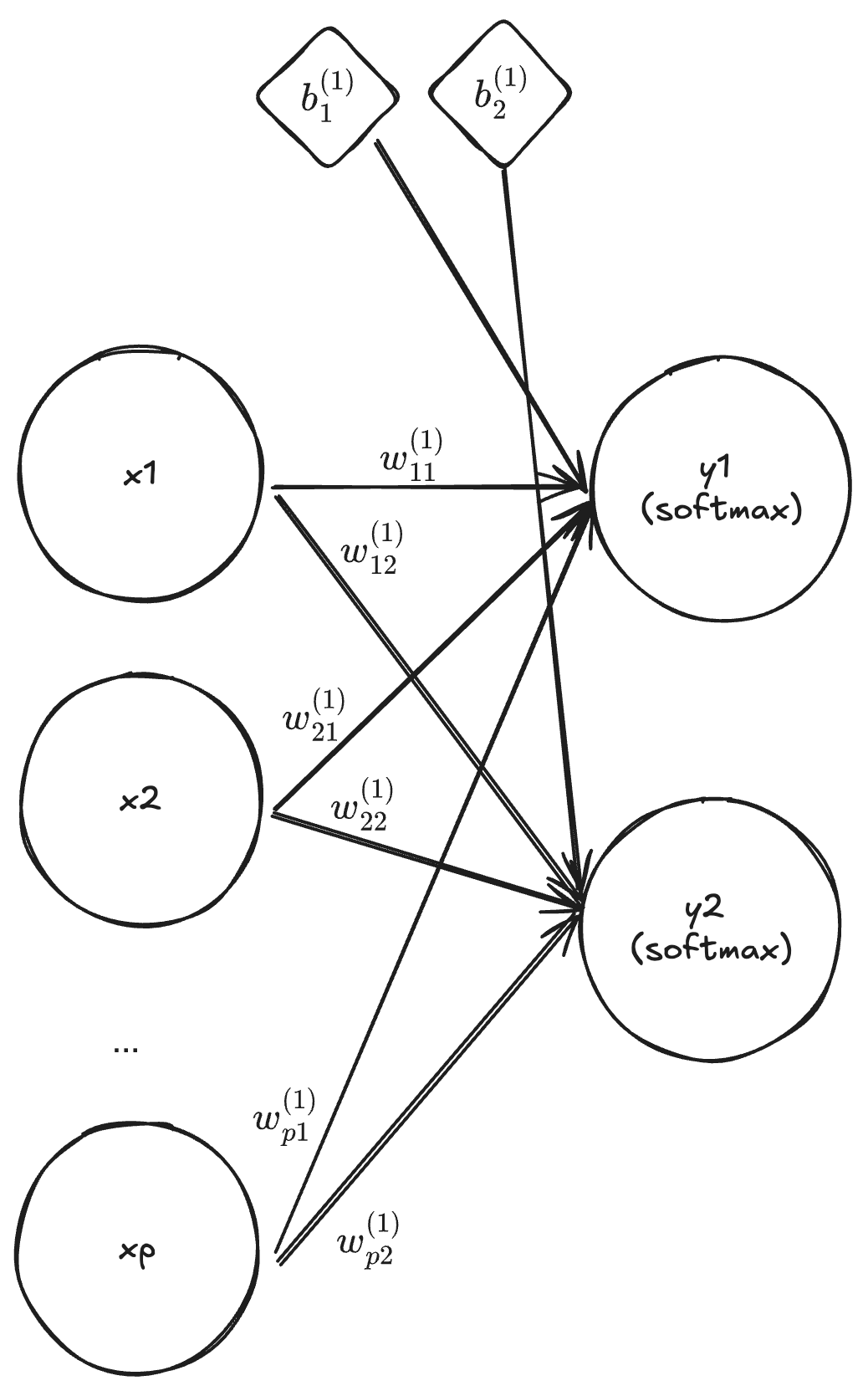
Multinomial logistic regression

By setting the dimension of \mathbb{x} to p, the dimension of \mathbf{y} and \mathbf{b}_1 to K, L = 1 and f^{(1)}(\mathbf{z}) = \frac{\exp(\mathbf{z})}{\sum_{k=1}^{K}\exp({z_k})}, we obtain

\mathbf{y} = f^{(1)}(\mathbf{W}^{(1)} \mathbf{x} + \mathbf{b}^{(1)}) = \frac{\exp(\mathbf{W}^{(1)} \mathbf{x} + \mathbf{b}^{(1)})}{\sum_{k=1}^{K} \exp\big(\mathbf{W}^{(1)} \mathbf{x} + b^{(1)}_{k}\big)}.

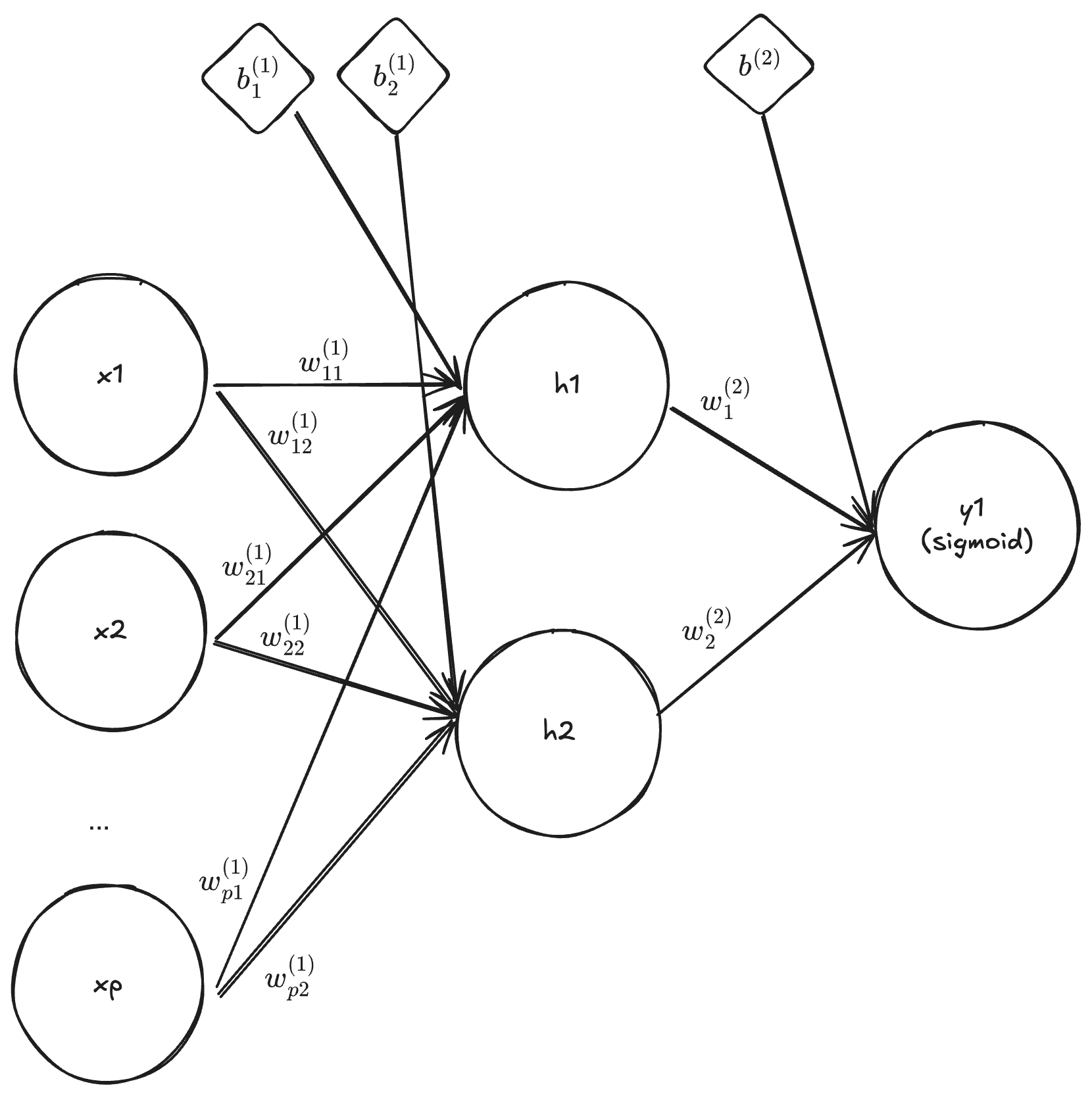
Multi-layer binary classifier

By setting the dimension of \mathbb{x} to p, the dimension of \mathbf{y} and \mathbf{b}_1 to one, L = 2, f^{(1)}(z) = z and f^{(2)}(\mathbf{z}) = \frac{\exp(\mathbf{z})}{\sum_{k=1}^{K}\exp({z_k})}, we obtain

\mathbf{h} = \mathbf{w}^{(1)} \mathbf{x} + \mathbb{b}^{(1)}, \quad \mathbf{y} = f^{(2)}(\mathbf{W}^{(2)} \mathbf{h} + b^{(2)}) = \frac{e^{\mathbf{W}^{(2)} \mathbf{h} + b^{(2)}}}{1 + e^{\mathbf{W}^{(2)} \mathbf{h} + b^{(2)}}}.

Activation functions

• Linear:
  • f(x) = x
  • f'(x) = 1
• Sigmoid:
  • f(x) = \frac{1}{1 + \exp(-x)}
  • f'(x) = f(x)[1 - f(x)]
• Tanh:
  • f(x) = \frac{\exp(x) - \exp(-x)}{\exp(x) + \exp(-x)}
  • f'(x) = 1 - [f(x)]^2

• ReLU (Rectified Linear Unit):
  • f(x) = \max(0, x)
  • f'(x) = \begin{cases} 1, & x > 0 \\ 0, & x \le 0 \end{cases}
• Softmax:
  • f(\mathbf{x}) = \frac{\exp(\mathbf{x})}{\mathbf{1}^\top\exp(\mathbf{x})}
  • \nabla_{\mathbf{x}} \mathbf{f}(\mathbf{x}) = \text{diag}(\mathbf{f}(\mathbf{x})) - \mathbf{f}(\mathbf{x}) \mathbf{f}(\mathbf{x})^\top

Neural network topology

You can choose:

• Number of layers (input, hidden, output)
• Number of units in each hidden layer
• Activation function for each layer, or even for individual units (though uncommon)
• Connection pattern between layers (e.g., fully connected, convolutional, recurrent)
• Layer arrangement or branching, such as skip connections or parallel paths
• Output structure, depending on the task (single value, vector, or map)

Loss functions

Like many supervised learning methods, a neural network needs a differentiable loss function so that optimisers can compute gradients to update the model.

• Regression \hat{y} \in \mathbb{R}

  • Mean Squared Error (MSE): \frac{1}{N} (\mathbf{y} - \hat{\mathbf{y}})^\top (\mathbf{y} - \hat{\mathbf{y}})

  • Mean Absolute Error (MAE): \frac{1}{N} \sum_{i=1}^{N} |\hat{y}_i - y_i|

• Classification \hat{y} \in (0,1)

  • Categorical Cross-Entropy: -\frac{1}{N} \sum_{i=1}^{N} \sum_{k=1}^{K} y_{ik} \log(\hat{y}_{ik})

  • Kullback–Leibler Divergence: \sum_{k=1}^{K} y_k \log \frac{y_k}{\hat{y}_k}

  • Hinge Loss: \frac{1}{N} \sum_{i=1}^{N} \max(0, 1 - y_i \hat{y}_i)

• …

Backpropagation

Neural networks learn in the same way as other complex differentiable models, by iteratively updating parameters using gradients.

• Unlike linear regression, we cannot simply set the derivative of the loss to zero because the solution has no closed form.

• Computing gradients for all weights is highly nontrivial.

• The 1986 Backpropagation paper made this practical.

Backpropagation

The goal is to compute \frac{\partial L}{\partial \boldsymbol{W}} and \frac{\partial L}{\partial \boldsymbol{b}}.

Using the chain rule, this can be decomposed layer by layer as \frac{\partial L}{\partial W^{(l)}_{ij}} = \underbrace{\frac{\partial L}{\partial a^{(l)}_i}}_{\boldsymbol{?}} ~~ \underbrace{\frac{\partial a^{(l)}_i}{\partial z^{(l)}_i}}_{\substack{\text{gradient of }\\ \text{ activation } \\ \text{function} } } ~~ \underbrace{\frac{\partial z^{(l)}_i}{\partial W^{(l)}_{ij}}}_{\substack{\text{output of}\\ \text{layer}~ l-1}}, where W^{(l)}_{ij} is the weight between the j-th unit in layer l-1 and the i-th unit in layer l, z^{(l)}_i is the pre-activation input, and a^{(l)}_i is the activation output.

Backpropagation

To compute \frac{\partial L}{\partial a^{(l)}_i} recursively, we apply the chain rule through the next layer.

For l < L (hidden layers):

\frac{\partial L}{\partial a^{(l)}_i} = \sum_k W^{(l+1)}_{ki}~~ \underbrace{\frac{\partial L}{\partial a^{(l+1)}_k}}_{\text{recursive}} ~~\underbrace{\frac{\partial a^{(l+1)}_k}{\partial z^{(l+1)}_k}}_{\substack{\text{gradient of } \\ \text{activation} \\ \text{ function} }}

For l = L (output layer), \frac{\partial L}{\partial a^{(L)}_i} = \frac{\partial L}{\partial \hat{y}_i} which depends on the specific loss function used.

Backpropagation

Similarly, since \mathbf{b}^{(l)} contributes additively to \mathbf{z}^{(l)}, its gradient is simply

\frac{\partial L}{\partial b^{(l)}_i} = \frac{\partial L}{\partial a^{(l)}_i}~~ \underbrace{\frac{\partial a^{(l)}_i}{\partial z^{(l)}_i}}_{\substack{\text{gradient of} \\ \text{activation} \\ \text{function}}}.

By applying these relations backward from the output layer to the first, we can efficiently compute all gradients

Gradient descent

Gradient descent (GD) is an iterative method that updates model weights in the negative gradient direction to minimise a differentiable loss.

1. Feed forward to get \hat{y}_i, i=1,\dots,N
2. Compute gradient: \nabla L = \frac{1}{N}\sum_i \nabla L(\hat{y}_i,y_i)
3. Update weights: \boldsymbol{\theta}^{*} \leftarrow \boldsymbol{\theta} - \eta \nabla L

• Keep learning rate \eta small to avoid overshooting due to curvature

Stochastic gradient descent

Stochastic gradient descent (SGD) is a variant of gradient descent that updates weights using the gradient from a single (or a small batch of) sample(s) at each step.

1. Feed forward to get \hat{y}_i for i=1,\dots,N_b, with batch size N_b \in [1,N]
2. Compute gradient: \nabla L = \frac{1}{N_b}\sum_i \nabla L(\hat{y}_i,y_i)
3. Update weights: \boldsymbol{\theta}^{*} \leftarrow \boldsymbol{\theta} - \eta \nabla L

• Using smaller batches introduces noise but can help escape local minima
• Batch size N_b is a hyperparameter

Keras

Building neural networks in Keras

1. Set the Keras backend to PyTorch.

Sys.setenv(KERAS_BACKEND = "torch")
keras <- import("keras", convert = FALSE)
input <- keras$Input(tuple(32L, 32L, 3L))
x <- keras$layers$Flatten()(input)
x <- keras$layers$Dense(32L, activation = "relu")(x)
output <- keras$layers$Dense(1L, activation = "sigmoid")(x)
model <- keras$Model(input, output)

Building neural networks in Keras

2. Import Keras and disable automatic object conversion.

• This keeps the Python object in its original form.

Sys.setenv(KERAS_BACKEND = "torch")
keras <- import("keras", convert = FALSE)
input <- keras$Input(tuple(32L, 32L, 3L))
x <- keras$layers$Flatten()(input)
x <- keras$layers$Dense(32L, activation = "relu")(x)
output <- keras$layers$Dense(1L, activation = "sigmoid")(x)
model <- keras$Model(input, output)

Building neural networks in Keras

3. Define an input tensor with shape (H, W, C).

Sys.setenv(KERAS_BACKEND = "torch")
keras <- import("keras", convert = FALSE)
input <- keras$Input(tuple(32L, 32L, 3L))
x <- keras$layers$Flatten()(input)
x <- keras$layers$Dense(32L, activation = "relu")(x)
output <- keras$layers$Dense(1L, activation = "sigmoid")(x)
model <- keras$Model(input, output)

Building neural networks in Keras

4. Flatten the pixel values into a feature vector.

Sys.setenv(KERAS_BACKEND = "torch")
keras <- import("keras", convert = FALSE)
input <- keras$Input(tuple(32L, 32L, 3L))
x <- keras$layers$Flatten()(input)
x <- keras$layers$Dense(32L, activation = "relu")(x)
output <- keras$layers$Dense(1L, activation = "sigmoid")(x)
model <- keras$Model(input, output)

Building neural networks in Keras

5. Add a fully connected layer with 32 units and ReLU as activation function.

Sys.setenv(KERAS_BACKEND = "torch")
keras <- import("keras", convert = FALSE)
input <- keras$Input(tuple(32L, 32L, 3L))
x <- keras$layers$Flatten()(input)
x <- keras$layers$Dense(32L, activation = "relu")(x)
output <- keras$layers$Dense(1L, activation = "sigmoid")(x)
model <- keras$Model(input, output)

Building neural networks in Keras

6. Add an output layer with one unit and a sigmoid activation function.

Sys.setenv(KERAS_BACKEND = "torch")
keras <- import("keras", convert = FALSE)
input <- keras$Input(tuple(32L, 32L, 3L))
x <- keras$layers$Flatten()(input)
x <- keras$layers$Dense(32L, activation = "relu")(x)
output <- keras$layers$Dense(1L, activation = "sigmoid")(x)
model <- keras$Model(input, output)

Building neural networks in Keras

7. Create the model by specifying the input and output tensor.

Sys.setenv(KERAS_BACKEND = "torch")
keras <- import("keras", convert = FALSE)
input <- keras$Input(tuple(32L, 32L, 3L))
x <- keras$layers$Flatten()(input)
x <- keras$layers$Dense(32L, activation = "relu")(x)
output <- keras$layers$Dense(1L, activation = "sigmoid")(x)
model <- keras$Model(input, output)

Keras model summary

Data flow (# param): \text{Input} ~~\underbrace{\longrightarrow}_{0} ~~\text{Flatten}~~ \underbrace{\longrightarrow}_{3072 \times 32 + 32 = 98336} ~~\text{Hidden}~~ \underbrace{\longrightarrow}_{32 \times 1 + 1 = 33} ~~\text{Output}

model$summary()

Model: "functional"
┏━━━━━━━━━━━━━━━━━━━━━━━━━━━━━━━━━┳━━━━━━━━━━━━━━━━━━━━━━━━┳━━━━━━━━━━━━━━━┓
┃ Layer (type)                    ┃ Output Shape           ┃       Param # ┃
┡━━━━━━━━━━━━━━━━━━━━━━━━━━━━━━━━━╇━━━━━━━━━━━━━━━━━━━━━━━━╇━━━━━━━━━━━━━━━┩
│ input_layer (InputLayer)        │ (None, 32, 32, 3)      │             0 │
├─────────────────────────────────┼────────────────────────┼───────────────┤
│ flatten (Flatten)               │ (None, 3072)           │             0 │
├─────────────────────────────────┼────────────────────────┼───────────────┤
│ dense (Dense)                   │ (None, 32)             │        98,336 │
├─────────────────────────────────┼────────────────────────┼───────────────┤
│ dense_1 (Dense)                 │ (None, 1)              │            33 │
└─────────────────────────────────┴────────────────────────┴───────────────┘
 Total params: 98,369 (384.25 KB)
 Trainable params: 98,369 (384.25 KB)
 Non-trainable params: 0 (0.00 B)

Compile keras model

Once the model is defined, we specify its loss function and optimiser.

• Metrics (optional): Set performance metrics (do not need to be differentiable)

model$compile(loss = "binary_crossentropy",
              optimizer = "sgd",
              metrics = list("accuracy"))

Prepare training data

It is important to standardise the images so that their values are around 0, as modern weight initialisers expect this.

Convert R arrays to torch tensors with float32 data type:

x_train_mean <- mean(cat_and_dog$x_train)
x_train_sd <- sd(cat_and_dog$x_train)

x <- torch$tensor((cat_and_dog$x_train - x_train_mean)/x_train_sd,
                  dtype = torch$float32)
y <- torch$tensor(cat_and_dog$y_train, dtype = torch$float32)

x_test <- torch$tensor((cat_and_dog_test$x_test - x_train_mean)/x_train_sd,
                       dtype = torch$float32)
y_test <- torch$tensor(cat_and_dog_test$y_test, dtype = torch$float32)

Train Keras model

Train for 5 epochs (the model will see x five times):

history <- model$fit(x = x,
                     y = y, 
                     epochs = 5L, 
                     batch_size = 64L,
                     verbose = 2L)

Epoch 1/5
157/157 - 1s - 8ms/step - accuracy: 0.5737 - loss: 0.7175
Epoch 2/5
157/157 - 1s - 7ms/step - accuracy: 0.6250 - loss: 0.6496
Epoch 3/5
157/157 - 2s - 12ms/step - accuracy: 0.6470 - loss: 0.6254
Epoch 4/5
157/157 - 2s - 10ms/step - accuracy: 0.6659 - loss: 0.6081
Epoch 5/5
157/157 - 2s - 10ms/step - accuracy: 0.6737 - loss: 0.5960

Evaluate keras model

Prediction:

model$predict(x, verbose = 0L)

array([[0.17342566],
       [0.22466913],
       [0.3888184 ],
       ...,
       [0.0303942 ],
       [0.6031979 ],
       [0.6493077 ]], shape=(10000, 1), dtype=float32)

Train and test performance:

model$evaluate(x, y, verbose = 0L)

[0.60319584608078, 0.6758000254631042]

model$evaluate(x_test, y_test, verbose = 0L)

[0.6685400605201721, 0.6274999976158142]

What keras does under the hood?

1. Sets up torch tensors for us.
2. Performs the forward pass on these tensors \boldsymbol{X} \rightarrow \hat{\boldsymbol{y}}.
3. torch builds a computation graph to compute the loss L(\hat{\boldsymbol{y}},\boldsymbol{y}) and track gradients \nabla L(\hat{\boldsymbol{y}},\boldsymbol{y}).
4. keras updates the weights based on the gradients and optimiser settings \boldsymbol{\theta}^{*} \leftarrow \mathcal{O}(\boldsymbol{\theta}, \nabla L), then clears the gradients.

Other useful layers

Check the documentation: https://keras.io/api/layers/

• Dropout: randomly sets input units to 0 at a specified rate during training, while scaling the remaining active units by 1 / (1 - rate) to maintain the overall activation level.
• Concatenate: merges multiple inputs along a specified axis.
• GaussianNoise: adds random noise to inputs during training to improve generalisation.
• BatchNormalization: normalises its inputs over the batch, helping stabilise and speed up training.
• …

Exercises 2.1.2

1. Convert the training and test arrays in R to torch tensors.
2. Train a baseline model for 100 epochs with a single hidden layer of 64 units.
3. Extend the baseline by adding a dropout layer (rate = 0.3) and retrain.
4. Increase the hidden layer size to 256 units and retrain.
5. Add a second hidden layer along with dropout and retrain.
6. Train a three-hidden-layer model with 256 units per layer and dropout (0.3).
7. Use PCA-transformed features as input and train a model with 256 hidden units.
8. Compare the performance of all models with other machine learning methods.